Gen4565645644 AdministrationGen AdministrationGen AdministrationGen AdministrationGen AdministrationGen AdministrationGen AdministrationGen AdministrationGen AdministrationGen AdministrationGen AdministrationGen AdministrationGen AdministrationGen AdministrationGen AdministrationGen AdministrationGen AdministrationGen AdministrationGen AdministrationGen AdministrationGen AdministrationGen AdministrationGen AdministrationGen AdministrationGen AdministrationGen AdministrationGen AdministrationGen AdministrationGen AdministrationGen AdministrationGen AdministrationGen AdministrationGen AdministrationGen AdministrationGen AdministrationGen AdministrationGen AdministrationGen AdministrationGen AdministrationGen AdministrationGen AdministrationGen AdministrationGen AdministrationGen AdministrationGen AdministrationGen AdministrationGen AdministrationGen AdministrationGen AdministrationGen AdministrationGen AdministrationGen AdministrationGen AdministrationGen AdministrationGen AdministrationGen AdministrationGen AdministrationGen AdministrationGen AdministrationGen AdministrationGen AdministrationGen AdministrationGen AdministrationGen AdministrationGen AdministrationGen AdministrationGen AdministrationGen AdministrationGen AdministrationGen AdministrationGen AdministrationGen AdministrationGen AdministrationGen AdministrationGen AdministrationGen AdministrationGen AdministrationGen AdministrationGen AdministrationGen AdministrationGen AdministrationGen AdministrationGen AdministrationGen AdministrationGen AdministrationGen AdministrationGen AdministrationGen AdministrationGen AdministrationGen AdministrationGen AdministrationGen AdministrationGen AdministrationGen AdministrationGen AdministrationGen AdministrationGen AdministrationGen AdministrationGen AdministrationGen AdministrationGen AdministrationGen AdministrationGen AdministrationGen AdministrationGen AdministrationGen AdministrationGen AdministrationGen AdministrationGen AdministrationGen AdministrationGen AdministrationGen AdministrationGen AdministrationGen AdministrationGen AdministrationGen AdministrationGen AdministrationGen AdministrationGen AdministrationGen AdministrationGen AdministrationGen AdministrationGen AdministrationGen AdministrationGen AdministrationGen AdministrationGen AdministrationGen AdministrationGen AdministrationGen AdministrationGen AdministrationGen AdministrationGen AdministrationGen AdministrationGen AdministrationGen AdministrationGen AdministrationGen AdministrationGen AdministrationGen AdministrationGen AdministrationGen AdministrationGen AdministrationGen AdministrationGen AdministrationGen AdministrationGen AdministrationGen AdministrationGen AdministrationGen AdministrationGen AdministrationGen AdministrationGen AdministrationGen AdministrationGen AdministrationGen AdministrationGen AdministrationGen AdministrationGen AdministrationGen AdministrationGen AdministrationGen AdministrationGen AdministrationGen AdministrationGen AdministrationGen AdministrationGen AdministrationGen AdministrationGen AdministrationGen AdministrationGen AdministrationGen AdministrationGen AdministrationGen Administrationv

ManagementManagementManagementManagementManagementManagementManagementManagement

ManagementManagementManagementManagement4545

ManagementManagementManagementManagementManagementManagementManagementManagement

ManagementManagementManagementManagementManagement

testsdfsdfdsfds

Lorem ipsum dolor sit amet, consectetur adipiscing elit. Nunc ac faucibus odio. Vestibulum neque massa, scelerisque sit amet ligula eu, congue molestie mi. Praesent ut varius sem. Nullam at porttitor arcu, nec lacinia nisi. Ut ac dolor vitae odio interdum condimentum. Vivamus dapibus sodales ex, vitae malesuada ipsum cursus convallis. Maecenas sed egestas nulla, ac condimentum orci. Mauris diam felis, vulputate ac suscipit et, iaculis non est. Curabitur semper arcu ac ligula semper, nec luctus nisl blandit. Integer lacinia ante ac libero lobortis imperdiet. Nullam mollis convallis ipsum, ac accumsan nunc vehicula vitae. Nulla eget justo in felis tristique fringilla. Morbi sit amet tortor quis risus auctor condimentum. Morbi in ullamcorper elit. Nulla iaculis tellus sit amet mauris tempus fringilla. Maecenas mauris lectus, lobortis et purus mattis, blandit dictum tellus.  Maecenas non lorem quis tellus placerat varius.  Nulla facilisi.  Aenean congue fringilla justo ut aliquam.  Mauris id ex erat. Nunc vulputate neque vitae justo facilisis, non condimentum ante sagittis.  Morbi viverra semper lorem nec molestie.  Maecenas tincidunt est efficitur ligula euismod, sit amet ornare est vulputate. 12 10 0 2 4 6 8 Row 1 Row 2 Row 3 Row 4 Column 1 Column 2 Column 3 In non mauris justo. Duis vehicula mi vel mi pretium, a viverra erat efficitur. Cras aliquam est ac eros varius, id iaculis dui auctor. Duis pretium neque ligula, et pulvinar mi placerat et. Nulla nec nunc sit amet nunc posuere vestibulum. Ut id neque eget tortor mattis tristique. Donec ante est, blandit sit amet tristique vel, lacinia pulvinar arcu. Pellentesque scelerisque fermentum erat, id posuere justo pulvinar ut. Cras id eros sed enim aliquam lobortis. Sed lobortis nisl ut eros efficitur tincidunt. Cras justo mi, porttitor quis mattis vel, ultricies ut purus. Ut facilisis et lacus eu cursus. In eleifend velit vitae libero sollicitudin euismod. Fusce vitae vestibulum velit. Pellentesque vulputate lectus quis pellentesque commodo. Aliquam erat volutpat. Vestibulum in egestas velit. Pellentesque fermentum nisl vitae fringilla venenatis. Etiam id mauris vitae orci maximus ultricies. Cras fringilla ipsum magna, in fringilla dui commodo a. Lorem ipsum Lorem ipsum Lorem ipsum 1 In eleifend velit vitae libero sollicitudin euismod. Lorem 2 Cras fringilla ipsum magna, in fringilla dui commodo a. Ipsum 3 Aliquam erat volutpat. Lorem 4 Fusce vitae vestibulum velit. Lorem 5 Etiam vehicula luctus fermentum. Ipsum Etiam vehicula luctus fermentum. In vel metus congue, pulvinar lectus vel, fermentum dui. Maecenas ante orci, egestas ut aliquet sit amet, sagittis a magna. Aliquam ante quam, pellentesque ut dignissim quis, laoreet eget est. Aliquam erat volutpat. Class aptent taciti sociosqu ad litora torquent per conubia nostra, per inceptos himenaeos. Ut ullamcorper justo sapien, in cursus libero viverra eget. Vivamus auctor imperdiet urna, at pulvinar leo posuere laoreet. Suspendisse neque nisl, fringilla at iaculis scelerisque, ornare vel dolor. Ut et pulvinar nunc. Pellentesque fringilla mollis efficitur. Nullam venenatis commodo imperdiet. Morbi velit neque, semper quis lorem quis, efficitur dignissim ipsum. Ut ac lorem sed turpis imperdiet eleifend sit amet id sapien

RapidMiner: A No-Code Data Science Platform

What is RapidMiner?

RapidMiner is a data science platform that includes data mining tools and is popular with data scientists of all skill levels:

• Features

RapidMiner has a visual programming environment that supports the entire data science process, including data preparation, machine learning, data mining, and model deployment.

• User-friendly

RapidMiner has a user-friendly interface that makes it appealing to non-technical users.

• Data mining tools

RapidMiner's data mining tools include operators for association rule learning, clustering, text mining, and anomaly detection.

• Data preparation tools

RapidMiner's data preparation tools include operators for data cleaning, wrangling, and feature engineering.

• Machine learning tools

RapidMiner's machine learning tools include operators for supervised learning, unsupervised learning, and reinforcement learning.

• Model deployment tools

RapidMiner's model deployment tools help you deploy predictive analytics models to production environments

RapidMiner is a data science platform that provides a visual programming environment for developing and deploying predictive analytics applications. It is a popular choice for data scientists of all skill levels, but it is especially appealing to non-technical users due to its user-friendly interface and wide range of features.

RapidMiner offers a variety of features that support the entire data science process, from data preparation to modelling to validation. These features include:

• Data preparation: RapidMiner offers a variety of operators for data cleaning, wrangling, and feature engineering.
• Machine learning: RapidMiner offers a variety of operators for supervised learning, unsupervised learning, and reinforcement learning.
• Data mining: RapidMiner offers a variety of operators for association rule learning, clustering, text mining, and anomaly detection.
• Model deployment: RapidMiner offers a variety of features for deploying predictive analytics models to production environments.

RapidMiner also offers a number of features that make it particularly appealing to non-technical users, such as:

• Visual programming interface: RapidMiner’s visual programming interface makes it easy to create and modify data science workflows without having to write any code.
• Pre-built operators: RapidMiner includes a library of pre-built operators that can be used to perform common data science tasks.
• Drag-and-drop functionality: RapidMiner’s drag-and-drop functionality makes it easy to create and modify data science workflows.
• Interactive visualization: RapidMiner offers interactive visualization tools that allow users to explore their data and visualize the results of their analysis.
• Collaboration features: RapidMiner includes collaboration features that allow users to share and collaborate on data science projects.

RapidMiner is a powerful and versatile data science platform that is well-suited for users of all skill levels. Its user-friendly interface, wide range of features, and pre-built operators make it a particularly good choice for non-technical users who are looking to get started with data science.

Here are some of the benefits of using RapidMiner:

• Increased productivity: RapidMiner’s visual programming interface and pre-built operators can help users to be more productive by eliminating the need to write code and switch between multiple tools.
• Improved accuracy: RapidMiner’s features for data preparation, model selection, and model validation can help users improve the accuracy of their predictive analytics models.
• Reduced costs: RapidMiner’s open-source license and its ability to automate data science workflows can help users reduce the cost of developing and deploying predictive analytics applications.

Getting Started with RapidMiner

Installation:

• Download RapidMiner Studio from the official RapidMiner website.
• Install RapidMiner Studio on your computer, following the installation guide provided during the download process.

Familiarize Yourself with the Interface:

Interface

Repository Panel

The Repository Panel in RapidMiner Studio is essentially the central storage area for all the objects you create or import. Here’s what it contains:

• Data: You can store various data sets in the repository. These could be in different formats like Excel, CSV, databases, or data generated through RapidMiner processes.
• Processes: This is where the analytical procedures that you have created are saved. A process is a sequence of operations performed on data to achieve a specific goal, such as data cleaning, transformation, analysis, or model building.
• Models: Once a predictive model has been created and trained, it can be saved in the repository. Saved models can be applied to new data or further refined at a later stage.
• Results: The output from processes, such as charts, statistics, or predictions, is stored here. These results can be viewed at any time and can be used for reports or presentations.
• Extensions: RapidMiner can be extended with additional functionality through extensions which are also stored in the repository once installed.

Users manage their projects by organizing these items into folders within the Repository Panel, making it easier to navigate and manage large numbers of files.

Process Panel

The Process Panel is where you design and build your data analysis workflows in RapidMiner Studio. This panel represents the workspace or canvas for crafting an analytical process. Here’s how it works:

• Designing Workflows: You create a workflow by dragging and dropping operators from the Operators Panel onto the Process Panel. Operators are the building blocks of any process in RapidMiner and can perform a variety of functions, from simple data transformations to complex predictive analytics.
• Connecting Operators: Operators are connected with ‘ports’ that define the flow of data from one operation to the next. These connections are represented as arrows, visually indicating the sequence of operations.
• Executing Processes: Once the operators are connected, you can run the entire process or step through it one operator at a time to debug or understand intermediate steps.
• Modifying Workflows: You can easily modify a workflow by adding, removing, or rearranging operators to optimize or adjust the analysis process.

Operators Panel

The Operators Panel is a comprehensive library of all the operators available in RapidMiner. It’s categorized to help you find the right tool for the job:

• Search Function: You can use the search bar to find operators by name or functionality. This is helpful if you know what task you want to perform but not the specific operator name.
• Categorization: Operators are organized into groups based on their function, such as ‘Blending’, ‘Cleaning’, ‘Modeling’, ‘Evaluation’, and ‘Visualization’, among others.
• Operator Information: By clicking on an operator or hovering over it, you get information about what it does, the inputs it requires, the outputs it produces, and the configuration parameters it accepts.

Parameters Panel

When you select an operator in the Process Panel, the Parameters Panel displays settings that can be adjusted to customize the operator’s behavior:

• Configurable Options: The panel shows all the configurable options for the selected operator, including paths to data sets, algorithm parameters, and display settings.
• Dynamic Adjustment: As you change parameter values, RapidMiner might dynamically update other options or provide feedback on the validity of the entered values.
• Expert Settings: Some operators have ‘expert’ settings available that can be accessed by enabling the ‘Show advanced parameters’ option. These settings provide finer control over the operator’s function but require a deeper understanding of the operator’s role within the process.

Importing Data

Importing data

Preprocessing Data

Include more operators for data preprocessing(based on your data set and the requirements

More about Operators

RapidMiner operators are the building blocks of data science workflows. They are responsible for performing specific tasks on data, such as cleaning, transforming, and modelling. Operators are connected together to create workflows that perform complex data analysis and machine learning tasks.

Operators have a specific structure, which is defined by the following parameters:

• Name: The unique name of the operator.
• Description: A brief description of what the operator does.
• Input ports: The ports that receive input data.
• Output ports: The ports that output processed data.
• Parameters: The parameters that control how the operator operates.

Operators can be classified into different types, such as:

• Data preparation operators: These operators perform tasks such as data cleaning, wrangling, and feature engineering.
• Machine learning operators: These operators perform tasks such as model training, evaluation, and prediction.
• Data mining operators: These operators perform tasks such as association rule learning, clustering, text mining, and anomaly detection.
• Model deployment operators: These operators deploy predictive analytics models to production environments.

RapidMiner also offers a number of special operators, such as:

• Meta operators: These operators control the flow of data through a workflow.
• Iterators: These operators repeat a workflow multiple times with different inputs.
• Custom operators: These operators are created by users to perform specific tasks that are not available in the built-in operator library.

Operators can be combined together to create complex data science workflows. For example, a workflow might include operators for data cleaning, feature engineering, model training, and model evaluation.

Here is an example of a simple RapidMiner workflow:

Read File -> Select Attributes -> Normalize -> Train Model -> Evaluate Model

This workflow reads a data file, selects a subset of attributes, normalizes the data, trains a machine learning model, and evaluates the model.

Operators can be organized into groups and sub-groups to make them easier to manage. For example, the machine learning operators could be organized into a group called “Machine Learning”, and the data preparation operators could be organized into a group called “Data Preparation”.

Operators can also be parameterized to customize their behaviour. For example, the “Normalize” operator has a parameter called “Normalization Method” that can be used to choose the normalization method to use.

RapidMiner’s operator architecture is flexible and powerful. It allows users to create complex data science workflows without having to write any code.

Once you have dragged and dropped operators into the Process Panel in RapidMiner, you’ll need to connect them to build a data analysis workflow. Here’s how you can complete the task using ports and other features:

Connecting Operators with Ports

Each operator has input and output ports, which appear as small squares or rectangles on the left (input) and right (output) sides of the operator’s block. To build a functioning process, you must connect the output port of one operator to the input port of the subsequent operator in your workflow.

Here’s a step-by-step guide to connecting operators:

1. Identify Ports: First, take a look at the ports on your chosen operators. Ports are colour-coded and labelled to help you understand their purpose. For example, blue ports are typically used for data input and output, while other colours may represent different types of inputs and outputs such as models, performance vectors, or charts.
2. Create a Connection: Click on the output port of the first operator, then drag your mouse pointer to the input port of the next operator you want to connect to. Release the mouse button to establish the connection. A line (or ‘noodle’) will appear, showing the data flow between operators.
3. Configure Operators: Click on an operator to select it, which will bring up its configurable parameters in the Parameters Panel. Set the appropriate parameters for the task that the operator is supposed to perform. For example, if you’re using a ‘Read CSV’ operator, you would specify the file path and import settings such as column separators, data types for each column, and whether the first row contains column names.
4. Sequence Your Process: Continue connecting operators in sequence to build your process. Often, you’ll need to follow a typical data processing sequence: data input → data preprocessing → data transformation → modelling → output.
5. Branching and Merging: Some processes might require branching (using one dataset in multiple ways) or merging (combining multiple datasets into one). This can be done by connecting one operator’s output to multiple inputs or vice versa.
6. Nested Processes: For more complex tasks, you can use ‘Subprocess’ operators to create nested workflows. This helps keep your main process clean and organized.

Connecting Ports

1. Running the Process: After setting up your workflow, you can run the entire process by clicking the ‘Run’ button (play icon) at the top of the screen. Alternatively, you can right-click an operator and select ‘Run to here’ to execute the process up to that point.
2. Viewing Results: Once the process runs, you can view the results in the Results Panel. If the process includes a modelling operator followed by an application and performance evaluation, you’ll see the model’s performance metrics, such as accuracy or ROC curve, displayed here.
3. Debugging: If there are errors or the process does not produce the expected results, check the connections between operators, ensure all parameters are set correctly, and look for error messages in the log panel. RapidMiner provides detailed error messages that can help pinpoint what went wrong.
4. Iteration and Optimization: Analyze the results, and if necessary, return to your process to make adjustments. You can add, remove, or replace operators, tweak their parameters, or try different modelling techniques to optimize performance.

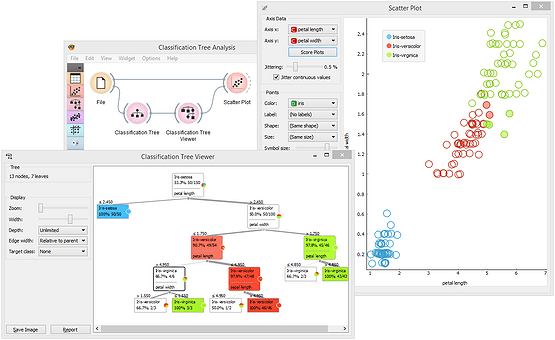
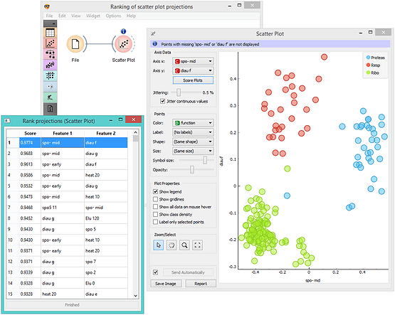
Results

Here’s the algorithm selection. Rapidminer will serve several popular classification algorithms for us to choose from.

This is the list of algorithms you can choose:

1. Naive Bayes
2. Generalized Linear Model
3. Logistic Regression
4. Fast Large Margin
5. Deep Learning
6. Decision Tree
7. Random Forest
8. Gradient Boosted Trees
9. Support Vector Machine

RapidMiner is a comprehensive data science platform that caters to both seasoned data scientists and beginners. Here are its key features:

1. Visual Workflow Design:
   • RapidMiner’s strength lies in its visual interface. Instead of writing code, you build workflows by dragging and dropping components onto a canvas.
   • This approach makes it accessible to non-developers who want to explore data, create models, and gain insights without diving into programming.
2. Machine Learning Libraries:
   • The platform provides pre-defined machine learning libraries, including text analytics, predictive modeling, clustering, and more.
   • You can also integrate third-party libraries, giving you flexibility in your analyses.
3. No Coding Required:
   • Whether you’re analyzing data, preprocessing, or building models, RapidMiner allows you to do it all without writing complex code.
   • It’s like having a data science assistant that speaks your language!

Using RapidMiner: A Practical Example

Let’s walk through a simple case study using RapidMiner:

1. Accessing the Samples Repository:
   • When you open RapidMiner Studio, you’ll find a built-in samples repository. It’s a treasure trove of practice exercises.
   • The repository contains both sample data sets and sample processes.
2. Sample Data Sets:
   • In the “data” folder, you’ll discover various data sets. These datasets cover different types of data, allowing you to practice with diverse examples.
3. Sample Processes:
   • The “processes” folder contains over 130 sample workflows. These processes demonstrate various tasks, such as preprocessing, visualization, and clustering.
   • Each process is organized by function, making it easy to explore specific topics.
   • You have two ways to use these processes:
     • Double-Click Method:
       • Double-click on a process to view its individual operators. Each operator comes with explanatory help text.
       • This method is excellent for learning and understanding how different components fit together.
     • Drag-and-Drop Method:
       • Drag a process onto the canvas. RapidMiner automatically creates an “Execute” operator.
       • The Execute operator runs the entire process.
       • Connect the results port to see the output.
       • This method is efficient once you’re familiar with the process.
4. Structuring Your Workflows:
   • As you gain experience, save multi-operator processes to the repository.
   • For example, create separate processes for data updating, preprocessing, model creation, and performance checks.
   • Then, in your main workflow, use interconnected Execute operators for a neat and tidy design.

-----------------------------------------------------------------------------------------------------------------------------------

What is Orange?

• Overview: Orange is an open-source data science platform that empowers users to perform various tasks without writing code. It combines visual workflow design with powerful functionality.
• Widgets: In Orange, the basic building blocks are called “widgets.” These widgets represent different data mining operations and can be connected to create workflows.
• Visual Programming: Instead of coding, you build your data analysis pipelines by connecting widgets on a canvas. It’s like creating a flowchart for your data!
• Orange Data Mining
• Orange is a C++ core object and routines library that incorporates a huge variety of standard and non-standard machine learning and data mining algorithms. It is an open-source data visualization, data mining, and machine learning tool. Orange is a scriptable environment for quick prototyping of the latest algorithms and testing patterns. It is a group of python-based modules that exist in the core library. It implements some functionalities for which execution time is not essential, and that is done in Python.

• It incorporates a variety of tasks such as pretty-print of decision trees, bagging and boosting, attribute subset, and many more. Orange is a set of graphical widgets that utilizes strategies from the core library and orange modules and gives a decent user interface. The widget supports digital-based communication and can be gathered together into an application by a visual programming tool called an orange canvas.
• All these together make an orange an exclusive component-based algorithm for data mining and machine learning. Orange is proposed for both experienced users and analysts in data mining and machine learning who want to create and test their own algorithms while reusing as much of the code as possible, and for those simply entering the field who can either write short python contents for data analysis.
• The objective of Orange is to provide a platform for experiment-based selection, predictive modeling, and recommendation system. It primarily used in bioinformatics, genomic research, biomedicine, and teaching. In education, it is used for providing better teaching methods for data mining and machine learning to students of biology, biomedicine, and informatics.

Orange Data Mining:

Orange supports a flexible domain for developers, analysts, and data mining specialists. Python, a new generation scripting language and programming environment, where our data mining scripts may be easy but powerful. Orange employs a component-based approach for fast prototyping. We can implement our analysis technique simply like putting the LEGO bricks, or even utilize an existing algorithm. 

What are Orange components for scripting Orange widgets for visual programming?. Widgets utilize a specially designed communication mechanism for passing objects like classifiers, regressors, attribute lists, and data sets permitting to build easily rather complex data mining schemes that use modern approaches and techniques.

• Orange core objects and Python modules incorporate numerous data mining tasks that are far from data preprocessing for evaluation and modeling. The operating principle of Orange is cover techniques and perspective in data mining and machine learning. For example, Orange's top-down induction of decision tree is a technique build of numerous components of which anyone can be prototyped in python and used in place of the original one. Orange widgets are not simply graphical objects that give a graphical interface for a specific strategy in Orange, but it includes an adaptable signaling mechanism that is for communication and exchange of objects like data sets, classification models, learners, objects that store the results of the assessment. All these ideas are significant and together recognize Orange from other data mining structures.

Orange Widgets:

• Orange widgets give us a graphical user interface to orange's data mining and machine learning techniques. They incorporate widgets for data entry and preprocessing, classification, regression, association rules and clustering a set of widgets for model assessment and visualization of assessment results, and widgets for exporting the models into PMML.( Predictive Model Markup Language)

• Widgets convey the data by tokens that are passed from the sender to the receiver widget. For example, a file widget outputs the data objects, that can be received by a widget classification tree learner widget. The classification tree builds a classification model that sends the data to the widget that graphically shows the tree. An evaluation widget may get a data set from the file widget and objects.

Orange scripting:

• If we want to access Orange objects, then we need to write our components and design our test schemes and machine learning applications through the script. Orange interfaces to Python, a model simple to use a scripting language with clear and powerful syntax and a broad set of additional libraries. Same as any scripting language, Python can be used to test a few ideas mutually or to develop more detailed scripts and programs.

Key Features of Orange:

1. Visual Workflow Design:
   • Widgets are the heart of Orange. You drag and drop them onto the canvas to create your analysis pipeline.
   • For example, the File widget reads data from a file, and the Data Table widget displays the data in a spreadsheet format. You connect them to load and visualize your data¹.
2. Interactive Visualizations:
   • Most visualizations in Orange are interactive. Take the Scatter Plot widget, for instance.
   • Double-click its icon to open it, and then click-and-drag to select data points directly from the plot.
   • The selected data automatically propagates to the Data Table widget, where you can inspect which data was chosen.
   • It’s a seamless way to explore relationships between variables and understand your data¹.
3. Pivot Table:
   • The Pivot Table widget helps aggregate and transform data. You can use it to summarize information based on specific criteria.
   • For example, aggregate Kickstarter projects by month and compare funded vs. non-funded projects.
   • Experiment with different aggregation methods to gain insights¹.
4. Classification Tree Visualization:
   • Combine the interface and visualization of classification trees with the Scatter Plot widget.
   • When both the tree viewer and the scatter plot are open, selecting any node in the tree highlights related data instances in the scatter plot.
   • It’s like having an interactive classification tree browser at your fingertips¹.

Example: Sentiment Analysis Using Orange

Let’s walk through a practical example: sentiment analysis on a dataset of boat headphone reviews. We’ll use Orange’s no-code approach:

1. Data Loading:
   • Start with the File widget to read your dataset.
   • Connect it to the Data Table widget to visualize the data.
2. Text Mining:
   • Use widgets like Text Preprocessing and Bag of Words to prepare the text data.
   • Create a sentiment label (positive/negative) based on review content.
3. Model Building:
   • Connect widgets like Naive Bayes or Random Forest to build a sentiment classification model.
4. Evaluation:
   • Evaluate the model’s performance using widgets like Confusion Matrix or ROC Curve.

Remember, Orange simplifies the entire process, allowing you to focus on insights rather than code.

Orange is a visual programming tool for data mining, machine learning, and data analysis. It's made up of components called widgets that can be combined to create workflows. Orange is user-friendly and has a visual interface that's suitable for beginners and experienced data miners alike. 

Here are some examples of what you can do with Orange: 

• Data visualization: Orange has interactive visualization tools like scatter plots, box plots, histograms, dendrograms, and silhouette plots. 
• Data exploration and preparation: Orange can help you reduce your data by selecting only the features you want to keep. 
• Feature engineering: Orange offers techniques for transforming and creating new features from existing data, such as feature scaling, discretization, and feature selection. 
• Text mining: Orange has tools for text preprocessing, topic modeling, sentiment analysis, and text classification. 
• Integration and extension: Orange lets you integrate your own Python scripts and custom Python code. 
• Add-ons: You can install additional widgets, or extensions, from the Options menu. 
• Interactive Data Visualization
• Orange is all about data visualizations that help to uncover hidden data patterns, provide intuition behind data analysis procedures or support communication between data scientists and domain experts. Visualization widgets include scatter plot, box plot and histogram, and model-specific visualizations like dendrogram, silhouette plot, and tree visualizations, just to mention a few. Many other visualizations are available in add-ons and include visualizations of networks, word clouds, geographical maps, and more.
• We take care to make Orange visualizations interactive: you can select data points from a scatter plot, a node in the tree, a branch in the dendrogram. Any such interaction will instruct visualization to send out a data subset that corresponds to the selected part of visualization. Consider the combination of a scatter plot and classification tree below. Scatter plot shows all the data, but highlights the data subset that corresponds to the selected node in the classification tree.
• 
• Great Visualizations
• Orange includes many standard visualizations. Scatter plot is great for visualizing correlations between pair of attributes, box plot for displaying basic statistics, heat map to provide an overview across entire data set, and projection plots like MDS(Multidimensional scaling is a technique which finds a low-dimensional (in our case a two-dimensional) projection of points, where it tries to fit distances between points as well as possible. The perfect fit is typically impossible to obtain since the data is high-dimensional or the distances are not Euclidean.) for plotting the multinomial data in two dimensions.
• 
• Besides visualizations one would expect in a data mining suite, Orange includes some great extras that you may not find in other packages. These include widgets for silhouette plot to analyze the results of clustering, mosaic and Sieve diagram to discover feature interactions, and Pythagorean tree visualization for classification trees and forests.
• 
• Exploratory Data Analysis
• Interactive visualizations enable exploratory data analysis. One can select interesting data subsets directly from plots, graphs and data tables and mine them in them downstream widgets. For example, select a cluster from the dendrogram of hierarchical clustering and map it to a 2D data presentation in the MDS plot. Or check their values of in the data table. Or observe the spread of its feature values in a box plot. Open all these windows at once and see how the changes in your selection affect other widgets. Or, for another example, cross-validate logistic regression on a data set and map some of the misclassifications to the two-dimensional projection. It is easy to turn Orange into a tool where domain experts can explore their data even if they lack insights in underlying statistics or machine learning.
• 
• Intelligent Visualizations
• Sometimes there are just too many choices. Say, when data has many features, which feature pair should we visualize in a scatter plot to provide most information? Intelligent visualization comes to the rescue! In Orange's scatter plot, this is called Score Plots. When class information is provided, Score Plots finds projections with best class separation. Consider brown-selected data set (comes with Orange) and its 79 features. There are 3,081 (79*78/2) different features pairs, way too many to check them manually, but there are only a few feature combinations that yield a great scatter plot. Score Plots finds them all, and allows us to browse through them.
• 
• Reporting
• Finally, we can include the most important visualizations, statistics and information about the models into the report with a single click. Orange includes clever reporting where you can access workflow history for every widget and visualization directly from the report.
• 

·

Introducing a No-Code tool for Data Scientists to teach beginners how to create their first machine learning models without coding experience.

Nowadays everyone is talking about Artificial Intelligence and Data Science, especially after the latest results obtained by the Generative AI.
There are plenty of sources from which to acquire information useful for learning the basics of AI: newspaper articles, posts on various social networks, video interviews with experts in the field, and much more.

However, going from theory to practice is not so trivial, especially if you do not have a good foundation in computer programming.

Imagine having to use this tool to teach a person unfamiliar with the basics of data science and artificial intelligence to develop his/her first model.

It would be utopian to think of obtaining results by starting with the use of this tool without giving a minimum theoretical basis on these topics.

Based both on the main features of Orange Data Mining and on the practical experience gained from preparing and delivering artificial intelligence courses for non-experts, these are the basic aspects to be considered as theoretical pre-requisites:

• History and basic definitions of Artificial Intelligence, Machine Learning and Data Science
• Machine Learning main application areas
• Machine Learning development steps: from data to value
• Based on the challenge you want to face, deep dive on the specific topic
  - Classification
  - Regression
  - NLP
  - Computer Vision
  - …

Ok, now you are ready: let’s install and configure our no-code tool!

How to install and configure Orange Data Mining

Orange Data Mining is a freely available visual programming software package that enables users to engage in data visualization, data mining, machine learning, and data analysis.
There are different ways to install this tool.
The easiest one is to access to the official website and download the Standalone installer.
If you already have the anaconda platform installed on your PC, you can also install orange as a package with the following commands:

• Anaconda: conda install -c conda-forge orange3
• Pip: pip install orange3

Orange Data Mining Interface

Well done!
Now you can start exploring Orange Data Mining.

Based on the installation mode there are two different ways to open the tool:

• If installed through the Standalone installer, you need to open the Orange application as a standard Windows app
• If installed as a Python library, you need the execute the following command: orange-canvas

Opening the tool interface will look like this.

Figure 1 — Orange Data Mining Canvas

The popup enables you to initiate a new workflow from scratch or open an existing one.
Upon clicking the ‘New’ icon, a blank canvas is revealed.

To start populating this empty canvas, utilize the widgets [2], which serve as the computational units in Orange Data Mining.
Access them through the explorer bar on the left, conveniently organized into subgroups based on their functions:

• Data: for loading and storing data
• Transform: useful for data preparation and transformation
• Visualize: to create visualizations from data
• Model: for machine/deep learning models
• Evaluate: for evaluating the developed machine/deep learning model
• Unsupervised: includes models/techniques for an unsupervised approach

To employ these widgets, simply drag them from the explorer bar onto the canvas.
As an example, try dragging the File widget into the Data group; this widget aids in loading data from your hard drive.

The Orange Data Mining Interface will then adopt the following appearance:

Figure 2 — Orange Data Mining Widgets

You’ll notice that the widget features a dashed grey arch.
By clicking on it and dragging the mouse to the right, a line emerges from the widget. This line serves to connect two different widgets and kickstart the creation of your initial workflow.

The arch’s position relative to the widget provides insights into the widget’s requirements:

• One or more inputs: The arch is on the left of the widget.
• One or more outputs: The arch is on the right of the widget.
• Both inputs and outputs: the arch appears on both the left and right sides of the widget.

Armed with this information, you’re ready to delve into Orange!
To facilitate a better understanding of how to leverage this tool for developing a machine learning model, let’s dive into an example.

Load and Transform Data

You’ll be working with the Kaggle challenge titled ‘Red Wine Quality’ accessible at this link.

This dataset encompasses the characteristics of 1600 red and white variants of Portuguese ‘Vinho Verde’ wine, with the output variable representing a score between 0 and 10.

Our goal is to develop a classification model capable of predicting the score based on input features such as fixed acidity and citric acid.

To begin, download the dataset from the provided link and import it into Orange.
In the Data widget area, numerous options are available for loading and storing data.

In this instance, you can drag the CSV File Import widget onto our blank sheet. Double-click on it and select the ‘Red Wine Quality’ CSV file.

Figure 3 — Import a CSV in a workflow

Orange demonstrates the ability to automatically identify the CSV delimiter (in this case, a comma) and the column type for each column.

If any discrepancies are noted, you can address them by selecting a specific column and adjusting its type. After completing these adjustments, click ‘OK’ to close the widget pop-up.

To effectively utilize the dataset, it’s essential to establish a connection between the CSV input files and a widget designed for storing data in a tabular format. Drag the Data Table widget onto the canvas and connect the two widgets, as illustrated in the Figure 4.

Figure 4 — Create a Data Table

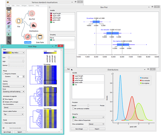
You can now explore into the dataset through some fundamental visualizations. Navigate to the explorer bar and locate the Visualize group. Drag and drop the Distributions, Scatter Plot, and Violin Plot widgets onto the canvas. Connect each of them to the Data Table for a comprehensive exploration.

Figure 5 — Basics of Data Visualization in Orange Data Mining

Take note of the text located above each link: to ensure that all data is visualized in your plots, it’s essential to double-click on the text and modify the link, as shown in the image below.

Figure 6 — How to use all data or a portion of a dataset

The Selected Data option proves useful when you wish to visualize (or, more broadly, inspect the results of your workflow) for only a subset of your dataset.
You can make this data selection by double-clicking on the Data Table and choosing a range of rows in a style reminiscent of Excel, as you can see in the Figure 7.

Figure 7 — Select a portion of a dataset

Now, let’s generate the target variable based on the quality feature. Suppose you want to setup a multiclass classification score, categorizing wine as bad if the quality is less than or equal to 4, medium for qualities between 5 and 6, and excellent otherwise.

To create the target column, use the Feature Constructor widget located in the Transform group (the widget has been renamed in the latest version of Orange to ‘Formula’).
Link the Data Table to this widget, and setting up the target column involves the following steps:

• Double-click on the widget
• Choose ‘categorical’ from the dropdown list
• Assign a name to the new variable (e.g., score)
• Specify the logical expression required; In this case:
  bad if quality<=4 else medium if quality <=6 else excellent
• Input bad, medium, excellent in the values field
• Click on Send (you will notice the rightmost icon below the button flashing)

Figure 8 — The Feature Constructor tool

To view the newly created column, connect a Data Table widget to the Feature Constructor, and double-click on it to inspect the added column.

Figure 9 — Data Preparation with Orange Data Mining

This is merely an illustrative example, so let’s move on. It’s worth noting that there are additional useful widgets in the Transform group for data preprocessing, such as merging and concatenating data, converting a column to continuous or discrete values, imputing missing values, and more.

Train and Evaluate the Models

First of all: although you’ve generated our ‘score’ variable, you haven’t designated it as the target yet.
The solution lies in the Select Column widget that you can see in the Figure 10.

Figure 10 — Select columns for a Machine Learning model

Now, our objective is to partition the dataset into Training Data and Test Data.

The Data Sampler widget facilitates this split, offering various methods and options (such as Stratify sample, crucial for addressing imbalanced classification problems).

Figure 11 — Split Train and Test Dataset

Now, let’s proceed to the modeling phase.

The most straightforward approach is to utilize the Test and Score widget within the Evaluate group.
This widget requires the following inputs:

• Training Data and Test Data: connect the Data Sampler to this widget, ensuring that the connections are configured as depicted in the image below.
• All the models you want to use add all the learners (you can find them in the tab “Model”) you wish to test onto our canvas and link each of them to the Test and Score widget.

Figure 12 — Test and Score different models

All the components are linked together. By opening the Test and Score widget, you can choose various training and test options and evaluate the performance of the tested models.

Figure 13 — Evaluate model performances

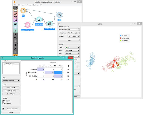
You can also examine the confusion matrix by connecting the output of the Test and Score widget to the Confusion Matrix widget.

Figure 14 — Visualize the Confusion Matrix

Task accomplished! The Figure 15 shows the complete (and simple) workflow that you have constructed step by step.

Figure 15 — The final workflow

Useful Extensions

The standard installation of Orange includes default widgets, but additional extensions are available for installation. The process of installing add-ons varies depending on the initial Orange installation type:

• In any installation mode, users can choose add-ons from the Options menu and add a new extension.
• If Orange is installed as a Python package, extensions can be added as separate packages. For example, to install text mining widgets, one can use the command: conda install -c conda-forge orange3-text.

Explore the complete widget catalog at this link.

Areas of application, advantages, limitations, and other tools

Orange Data Mining, with its user-friendly interface and open-source nature, presents several advantages that cater to a diverse range of users. Its visual programming interface stands out as an intuitive tool, allowing users with varying technical backgrounds to seamlessly create data analysis workflows. The richness of pre-built components, spanning data preprocessing, machine learning, and visualization, further enhances its appeal, providing users with a comprehensive toolkit for various data-related tasks.

Indeed, Orange is widely employed in academic settings to introduce students to the realms of data mining and machine learning, leveraging its user-friendly interface to make complex concepts more accessible.

However, Orange does have limitations. Scalability can be a concern, particularly when handling large datasets or complex workflows. The tool may not exhibit the same level of performance as some commercial alternatives in such scenarios. Additionally, while Orange offers a diverse array of machine learning algorithms, it might not incorporate the most cutting-edge or specialized models found in some proprietary tools.

In conclusion, Orange Data Mining stands out as a versatile and accessible tool, particularly for educational purposes and smaller to medium-sized datasets. Its strengths in visualization and community collaboration make it a valuable asset, but potential users should consider its scalability limitations and the learning curve associated with advanced features. The choice of Orange depends on the specific needs, preferences, and expertise of the user, with recognition of its contributions to the open-source data mining landscape.

------------------------------------------------------------------------------------------------------------------------

Data Mining in R: An Overview

The Power of R for Data Mining

R is a widely used programming language and environment for statistical computing and graphics. It provides a vast collection of packages and libraries specifically designed for data mining tasks. Here are some key reasons why R is a popular choice for data mining −

• Extensive Data Manipulation Capabilities − R offers powerful tools for data manipulation, transformation, and cleaning. With packages like dplyr and tidyr, users can easily filter, arrange, and reshape data to prepare it for mining.
• Rich Statistical Functionality − R comes with a comprehensive set of statistical functions and algorithms, allowing users to perform various analyses, such as regression, clustering, classification, and association rule mining. Packages like caret and randomForest provide implementations of popular algorithms.
• Visualization Tools − R provides excellent data visualization capabilities through packages like ggplot2 and plotly. These packages enable users to create visually appealing and informative plots, charts, and graphs to explore and present the results of their data mining analyses.
• Community Support and Active Development − R has a vibrant community of data scientists, statisticians, and developers who actively contribute to its growth. This ensures a continuous stream of new packages, updates, and resources for data mining tasks.

Data Mining Techniques in R

R offers a wide range of data mining techniques that can be applied to different types of datasets. Here are some commonly used techniques −

• Regression Analysis − Regression analysis is used to model the relationship between a dependent variable and one or more independent variables. R provides various regression models, such as linear regression, logistic regression, and polynomial regression, to analyze and predict numeric or categorical outcomes.
• Clustering − Clustering is a technique that groups similar data points together based on their characteristics or proximity. R offers algorithms like k-means, hierarchical clustering, and DBSCAN to perform clustering analysis and identify natural patterns or clusters within the data.
• Classification − Classification is used to categorize data into predefined classes or categories. R provides algorithms like decision trees, random forests, and support vector machines (SVM) for classification tasks. These algorithms can be trained on labeled data to predict the class of unseen instances.
• Association Rule Mining − Association rule mining is used to discover interesting relationships or associations between items in large datasets. R offers algorithms like Apriori and Eclat, which analyze transactional data and generate rules based on item co-occurrence patterns.

Practical Examples and Use Cases

Data mining with R finds applications in various domains. Here are a few examples −

• Market Basket Analysis − Retailers can use association rule mining to analyze customer purchase data and identify patterns like frequently co-purchased items. This information can be used for targeted marketing and product placement strategies.
• Fraud Detection − Data mining techniques like anomaly detection and classification can be employed to detect fraudulent activities in financial transactions, helping organizations prevent financial losses and maintain security.
• Customer Segmentation − Clustering algorithms can be used to group customers based on their behavior, preferences, or demographic characteristics. This segmentation enables organizations to tailor their marketing strategies and provide personalized experiences to different customer segments.
• Predictive Maintenance − By analyzing historical equipment data, data mining techniques can predict maintenance needs and potential failures in machinery. This helps businesses optimize maintenance schedules, minimize downtime, and reduce maintenance costs.

R Programming Tutorial

R Programming Tutorial is designed for both beginners and professionals.

R is a software environment which is used to analyze statistical information and graphical representation. R allows us to do modular programming using functions.

What is R Programming

"R is an interpreted computer programming language which was created by Ross Ihaka and Robert Gentleman at the University of Auckland, New Zealand." The R Development Core Team currently develops R. It is also a software environment used to analyze statistical information, graphical representation, reporting, and data modeling. R is the implementation of the S programming language, which is combined with lexical scoping semantics.

R not only allows us to do branching and looping but also allows to do modular programming using functions. R allows integration with the procedures written in the C, C++, .Net, Python, and FORTRAN languages to improve efficiency.

In the present era, R is one of the most important tool which is used by researchers, data analyst, statisticians, and marketers for retrieving, cleaning, analyzing, visualizing, and presenting data.

History of R Programming

The history of R goes back about 20-30 years ago. R was developed by Ross lhaka and Robert Gentleman in the University of Auckland, New Zealand, and the R Development Core Team currently develops it. This programming language name is taken from the name of both the developers. The first project was considered in 1992. The initial version was released in 1995, and in 2000, a stable beta version was released.

The following table shows the release date, version, and description of R language:

Features of R programming

R is a domain-specific programming language which aims to do data analysis. It has some unique features which make it very powerful. The most important arguably being the notation of vectors. These vectors allow us to perform a complex operation on a set of values in a single command. There are the following features of R programming:

1. It is a simple and effective programming language which has been well developed.
2. It is data analysis software.
3. It is a well-designed, easy, and effective language which has the concepts of user-defined, looping, conditional, and various I/O facilities.
4. It has a consistent and incorporated set of tools which are used for data analysis.
5. For different types of calculation on arrays, lists and vectors, R contains a suite of operators.
6. It provides effective data handling and storage facility.
7. It is an open-source, powerful, and highly extensible software.
8. It provides highly extensible graphical techniques.
9. It allows us to perform multiple calculations using vectors.
10. R is an interpreted language.

Why use R Programming?

There are several tools available in the market to perform data analysis. Learning new languages is time taken. The data scientist can use two excellent tools, i.e., R and Python. We may not have time to learn them both at the time when we get started to learn data science. Learning statistical modeling and algorithm is more important than to learn a programming language. A programming language is used to compute and communicate our discovery.

The important task in data science is the way we deal with the data: clean, feature engineering, feature selection, and import. It should be our primary focus. Data scientist job is to understand the data, manipulate it, and expose the best approach. For machine learning, the best algorithms can be implemented with R. Keras and TensorFlow allow us to create high-end machine learning techniques. R has a package to perform Xgboost. Xgboost is one of the best algorithms for Kaggle competition.

R communicate with the other languages and possibly calls Python, Java, C++. The big data world is also accessible to R. We can connect R with different databases like Spark or Hadoop.

In brief, R is a great tool to investigate and explore the data. The elaborate analysis such as clustering, correlation, and data reduction are done with R.

Comparison between R and Python

Data science deals with identifying, extracting, and representing meaningful information from the data source. R, Python, SAS, SQL, Tableau, MATLAB, etc. are the most useful tools for data science. R and Python are the most used ones. But still, it becomes confusing to choose the better or the most suitable one among the two, R and Python.

Applications of R

There are several-applications available in real-time. Some of the popular applications are as follows:

• Facebook
• Google
• Twitter
• HRDAG
• Sunlight Foundation
• RealClimate
• NDAA
• XBOX ONE
• ANZ
• FDA

Prerequisite

R programming is used for statistical information and data representation. So it is required that we should have the knowledge of statistical theory in mathematics. Understanding of different types of graphs for data representation and most important is that we should have prior knowledge of any programming.

Features of  R – Data Science

Some of the important features of R for data science applications are: 

• R provides extensive support for statistical modeling.
• R is a suitable tool for various data science applications because it provides aesthetic visualization tools.
• R is heavily utilized in data science applications for ETL (Extract, Transform, Load). It provides an interface for many databases like SQL and even spreadsheets.
• R also provides various important packages for data wrangling.
• With R, data scientists can apply machine learning algorithms to gain insights about future events.
• One of the important features of R is to interface with NoSQL databases and analyze unstructured data.

Most common R Libraries in Data Science

• Dplyr: For performing data wrangling and data analysis, we use the dplyr package. We use this package for facilitating various functions for the Data frame in R. Dplyr is actually built around these 5 functions. You can work with local data frames as well as with remote database tables. You might need to: 
  Select certain columns of data. 
  Filter your data to select specific rows. 
  Arrange the rows of your data in order. 
  Mutate your data frame to contain new columns. 
  Summarize chunks of your data in some way.
• Ggplot2: R is most famous for its visualization library ggplot2. It provides an aesthetic set of graphics that are also interactive. The ggplot2 library implements a “grammar of graphics” (Wilkinson, 2005). This approach gives us a coherent way to produce visualizations by expressing relationships between the attributes of data and their graphical representation.
• Esquisse: This package has brought the most important feature of Tableau to R. Just drag and drop, and get your visualization done in minutes. This is actually an enhancement to ggplot2. It allows us to draw bar graphs, curves, scatter plots, and histograms, then export the graph or retrieve the code generating the graph.
• Tidyr: Tidyr is a package that we use for tidying or cleaning the data. We consider this data to be tidy when each variable represents a column and each row represents an observation.
• Shiny: This is a very well-known package in R. When you want to share your stuff with people around you and make it easier for them to know and explore it visually, you can use Shiny. It’s a Data Scientist’s best friend.
• Caret: Caret stands for classification and regression training. Using this function, you can model complex regression and classification problems.
• E1071: The E1071 package has wide use for implementing clustering, Fourier Transform, Naive Bayes, SVM, and other types of miscellaneous functions.
• Mlr: This package is absolutely incredible in performing machine learning tasks. It almost has all the important and useful algorithms for performing machine learning tasks. It can also be termed as the extensible framework for classification, regression, clustering, multi-classification, and survival analysis.

Other worth mentioning R libraries: 

• Lubridate
• Knitr
• DT(DataTables)
• RCrawler
• Leaflet
• Janitor
• Plotly

Applications of R for Data Science

Top Companies that Use R for Data Science: 

• Google: At Google, R is a popular choice for performing many analytical operations. The Google Flu Trends project makes use of R to analyze trends and patterns in searches associated with flu.
• Facebook makes heavy use of R for social network analytics. It uses R for gaining insights about the behavior of the users and establishes relationships between them.
• IBM: IBM is one of the major investors in R. It recently joined the R consortium. IBM also utilizes R for developing various analytical solutions. It has used R in IBM Watson – an open computing platform.
• Uber: Uber makes use of the R package shiny for accessing its charting components. Shiny is an interactive web application that’s built with R for embedding interactive visual graphics.

R is another tool that is popular for data mining. R is an open-source programming tool developed by Bell Laboratories (formerly AT&T, now Lucent Technologies). Data scientists, machine learning engineers, and statisticians for statistical computing, analytics, and machine learning tasks prefer R

1. Getting Started with R:

• To begin data mining in R, you’ll need to install R itself and choose a development environment. One popular choice is RStudio, which provides a user-friendly interface for R.
• Once you have R and your preferred environment set up, you can start exploring the vast array of R packages and tools available for data mining.

2. Commonly Used R Packages for Data Mining:

Here are some essential R packages for data mining:

1. caret:
   • The caret package offers functions for training and evaluating machine learning models. It’s a go-to package for model selection, cross-validation, and hyperparameter tuning.
   • Example: You can use caret to train a classification model (e.g., logistic regression or random forest) on a dataset and evaluate its performance using metrics like accuracy or AUC.
2. dplyr:
   • dplyr provides a set of functions for data manipulation. It’s excellent for filtering, grouping, summarizing, and transforming data.
   • Example: You can use dplyr to filter rows based on specific conditions, group data by variables, and compute summary statistics.
3. ggplot2:
   • ggplot2 is a powerful data visualization package. It allows you to create a wide range of plots and charts.
   • Example: You can use ggplot2 to create scatter plots, bar charts, histograms, and more.
4. tm:
   • The tm package is specifically for text mining. It provides tools for preprocessing and analyzing text data.
   • Example: You can use tm to clean and tokenize text, create term-document matrices, and perform sentiment analysis.
5. igraph:
   • igraph is essential for analyzing and visualizing network data, including social networks, citation networks, and more.
   • Example: You can use igraph to explore relationships between nodes (e.g., users, websites, or genes) in a network.

3. Data Preparation (Data Preprocessing):

Before diving into data mining, you’ll need to prepare your data. Here are some common data preprocessing tasks in R:

• Reading Data:
  • Use the read.csv() function to read a CSV file into an R data frame.
• Reshaping Data:
  • The tidyr package provides functions like gather() and spread() for converting between wide and long data formats.
• Cleaning and Transforming Data:
  • dplyr comes in handy here. You can filter rows, create new variables, and handle missing values.

4. Example: Sentiment Analysis Using R:

Let’s walk through a practical example—sentiment analysis on a dataset of product reviews:

1. Data Loading:
   • Read the review data (e.g., from a CSV file) using read.csv().
   • Explore the structure of the data using str().
2. Text Mining:
   • Use the tm package to preprocess the text:
     • Remove stopwords (common words like “the,” “and,” etc.).
     • Tokenize the text (split it into words).
     • Create a document-term matrix.
   • Assign sentiment labels (positive/negative) based on the content.
3. Model Building:
   • Train a sentiment classification model (e.g., logistic regression or Naive Bayes) using caret.
   • Evaluate the model’s accuracy or other relevant metrics.
4. Visualization:
   • Use ggplot2 to create visualizations, such as bar charts showing sentiment distribution.

Remember, R is not only a programming language but also a powerful environment for data mining. 

Clustering is a technique used in data mining and machine learning to group similar data points together based on their attributes. It is an unsupervised learning method, meaning it doesn’t require predefined classes or labels. Clustering helps identify patterns and relationships in data, making it easier to analyze and understand large datasets.

Here are the main types of clustering methods in data mining:

1. Partitioning Clustering:
   • K-means Clustering: Divides the data into ( k ) clusters, where each data point belongs to the cluster with the nearest mean.
   • K-medoids Clustering: Similar to K-means but uses actual data points (medoids) as cluster centers.
2. Hierarchical Clustering:
   • Agglomerative (Bottom-Up): Starts with each data point as a single cluster and merges the closest pairs of clusters until only one cluster remains.
   • Divisive (Top-Down): Starts with all data points in one cluster and recursively splits them into smaller clusters.
3. Density-Based Clustering:
   • DBSCAN (Density-Based Spatial Clustering of Applications with Noise): Groups data points that are closely packed together, marking points in low-density regions as outliers.
   • OPTICS (Ordering Points To Identify the Clustering Structure): Similar to DBSCAN but can identify clusters of varying densities.
4. Grid-Based Clustering:
   • STING (Statistical Information Grid): Divides the data space into a grid structure and performs clustering on the grid cells.
   • CLIQUE (Clustering In QUEst): Combines grid-based and density-based approaches to find clusters in subspaces of high-dimensional data.
5. Model-Based Clustering:
   • Gaussian Mixture Models (GMM): Assumes that the data is generated from a mixture of several Gaussian distributions and uses the Expectation-Maximization (EM) algorithm to find the parameters of these distributions.
   • Hidden Markov Models (HMM): Used for clustering time-series data by modeling the data as a sequence of hidden states.
6. Fuzzy Clustering:
   • Fuzzy C-Means (FCM): Allows each data point to belong to multiple clusters with varying degrees of membership.

What is Clustering?

Different types of Clustering

Cluster Analysis separates data into groups, usually known as clusters. If meaningful groups are the objective, then the clusters catch the general information of the data. Some time cluster analysis is only a useful initial stage for other purposes, such as data summarization. In the case of understanding or utility, cluster analysis has long played a significant role in a wide area such as biology, psychology, statistics, pattern recognition machine learning, and mining.

The below diagram explains the working of the clustering algorithm. We can see the different fruits are divided into several groups with similar properties.

Clustering is the process of making a group of abstract objects into classes of similar objects.

Clustering is a technique used in machine learning to group similar data points together. It is an unsupervised learning method that does not require predefined classes or prior information.

Clustering helps to identify patterns and relationships in data that might be difficult to detect through other methods.

Clustering vs Classification -Classification is a supervised learning method that involves assigning predefined classes or labels to data points based on their features or attributes. In contrast, clustering is an unsupervised learning method that groups data points based on their similarities.

Points to Remember

• A cluster of data objects can be treated as one group.
• While doing cluster analysis, we first partition the set of data into groups based on data similarity and then assign the labels to the groups.

The main advantage of clustering over classification is that, it is adaptable to changes and helps single out useful features that distinguish different groups.

Cluster analysis, also known as clustering, is a method of data mining that groups similar data points together. The goal of cluster analysis is to divide a dataset into groups (or clusters) such that the data points within each group are more similar to each other than to data points in other groups. This process is often used for exploratory data analysis and can help identify patterns or relationships within the data that may not be immediately obvious. There are many different algorithms used for cluster analysis, such as k-means, hierarchical clustering, and density-based clustering. The choice of algorithm will depend on the specific requirements of the analysis and the nature of the data being analyzed.

Cluster Analysis is the process to find similar groups of objects in order to form clusters. It is an unsupervised machine learning-based algorithm that acts on unlabelled data. A group of data points would comprise together to form a cluster in which all the objects would belong to the same group.

The given data is divided into different groups by combining similar objects into a group. This group is nothing but a cluster. A cluster is nothing but a collection of similar data which is grouped together. 

For example, consider a dataset of vehicles given in which it contains information about different vehicles like cars,  buses, bicycles, etc. As it is unsupervised learning there are no class labels like Cars, Bikes, etc for all the vehicles, all the data is combined and is not in a structured manner.

• Clustering is a type of unsupervised learning that groups similar data points together based on certain criteria.
• The different types of clustering methods include Density-based, Distribution-based, Grid-based, Connectivity-based, and Partitioning clustering.
• Each type of clustering method has its own strengths and limitations, and the choice of method depends on the specific data analysis needs.
• Choosing the right clustering method and tools requires understanding your data, determining your goals, considering scalability, evaluating performance, and choosing the right tools.

Clustering is a powerful tool for data analysis that is a type of unsupervised learning that groups similar data points together based on certain criteria.

Now our task is to convert the unlabelled data to labelled data and it can be done using clusters.

The main idea of cluster analysis is that it would arrange all the data points by forming clusters like cars cluster which contains all the cars,  bikes clusters which contains all the bikes, etc.

Simply it is the partitioning of similar objects which are applied to unlabelled data.

Properties of Clustering :

1. Clustering Scalability: Nowadays there is a vast amount of data and should be dealing with huge databases. In order to handle extensive databases, the clustering algorithm should be scalable. Data should be scalable, if it is not scalable, then we can’t get the appropriate result which would lead to wrong results.

2. High Dimensionality: The algorithm should be able to handle high dimensional space along with the data of small size.

3. Algorithm Usability with multiple data kinds: Different kinds of data can be used with algorithms of clustering. It should be capable of dealing with different types of data like discrete, categorical and interval-based data, binary data etc.

4. Dealing with unstructured data: There would be some databases that contain missing values, and noisy or erroneous data. If the algorithms are sensitive to such data then it may lead to poor quality clusters. So it should be able to handle unstructured data and give some structure to the data by organising it into groups of similar data objects. This makes the job of the data expert easier in order to process the data and discover new patterns.

5. Interpretability: The clustering outcomes should be interpretable, comprehensible, and usable. The interpretability reflects how easily the data is understood.

What is Clustering in Data Mining?

Clustering in data mining is a technique that groups similar data points together based on their features and characteristics. It can also be referred to as a process of grouping a set of objects so that objects in the same group (called a cluster) are more similar to each other than those in other groups (clusters). It is an unsupervised learning technique that aims to identify similarities and patterns in a dataset. Clustering algorithms typically require defining the number of clusters, similarity measures, and clustering methods. These algorithms aim to group data points together in a way that maximizes similarity within the groups and minimizes similarity between different groups, as shown in the picture below.

Clustering techniques in data mining can be used in various applications, such as image segmentation, document clustering, and customer segmentation. The goal is to obtain meaningful insights from the data and improve decision-making processes.

What is a Cluster?

In data mining, a cluster refers to a group of data points with similar characteristics or features. These characteristics or features can be defined by the analyst or identified by the clustering algorithm while grouping similar data points together. The data points within a cluster are typically more similar to each other than those outside the cluster. For example, in the above figure, there are 5 clusters present.

A cluster can have the following properties -

• The data points within a cluster are similar to each other based on some pre-defined criteria or similarity measures.
• The clusters are distinct from each other, and the data points in one cluster are different from those in another cluster.
• The data points within a cluster are closely packed together.
• A cluster is often represented by a centroid or a center point that summarizes the properties of the data points within the cluster.
• A cluster can have any number of data points, but a good cluster should not be too small or too large.

Applications of Cluster Analysis

• Clustering analysis is broadly used in many applications such as market research, pattern recognition, data analysis, and image processing.
• Clustering can also help marketers discover distinct groups in their customer base. And they can characterize their customer groups based on the purchasing patterns.
• In the field of biology, it can be used to derive plant and animal taxonomies, categorize genes with similar functionalities and gain insight into structures inherent to populations.
• Clustering also helps in identification of areas of similar land use in an earth observation database. It also helps in the identification of groups of houses in a city according to house type, value, and geographic location.
• Clustering also helps in classifying documents on the web for information discovery.
• Clustering is also used in outlier detection applications such as detection of credit card fraud.
• As a data mining function, cluster analysis serves as a tool to gain insight into the distribution of data to observe characteristics of each cluster.

Market Segmentation

Market segmentation is the process of dividing a market into smaller groups of customers with similar needs or characteristics. Clustering can be used to identify such groups based on various factors such as demographics, behavior, and preferences.

Once the groups are identified, targeted marketing strategies can be developed to cater to their specific needs.

Clustering is a widely used technique in data mining and has numerous applications in various fields. Some of the common applications of clustering in data mining include -

• Customer Segmentation
  Clustering techniques in data mining can be used to group customers with similar behavior, preferences, and purchasing patterns to create more targeted marketing campaigns.
• Image Segmentation
  Clustering techniques in data mining can be used to segment images into different regions based on their pixel values, which can be useful for tasks such as object recognition and image compression.
• Anomaly Detection
  Clustering techniques in data mining can be used to identify outliers or anomalies in datasets that deviate significantly from normal behavior.
• Text Mining
  Clustering techniques in data mining can be used to group documents or texts with similar content, which can be useful for tasks such as document summarization and topic modeling.
• Biological Data Analysis
  Clustering techniques in data mining can be used to group genes or proteins with similar characteristics or expression patterns, which can be useful for tasks such as drug discovery and disease diagnosis.
• Recommender Systems
  Clustering techniques in data mining can be used to group users with similar interests or behavior to create more personalized recommendations for products or services.

Network Analysis

Clustering can also be used in network analysis to identify communities or groups of nodes with similar connectivity patterns.

Community detection algorithms use clustering techniques to identify such groups in social networks, biological networks, and other types of networks. This can help in understanding the structure and function of the network and in developing targeted interventions.

Anomaly Detection

Clustering can be used for anomaly detection, which is the process of identifying unusual or unexpected patterns in data.

Anomalies can be detected by clustering the data and identifying points that do not belong to any cluster or belong to a small cluster. This can be useful in fraud detection, intrusion detection, and other applications where unusual behavior needs to be identified.

Exploratory Data Analysis

Clustering can be used in exploratory data analysis to identify patterns and structures in data that may not be immediately apparent. This can help in understanding the data and in developing hypotheses for further analysis.

Clustering can also be used to reduce the dimensionality of the data by identifying the most important features or variables.

In summary, clustering is a versatile technique that can be applied to various domains such as market segmentation, network analysis, anomaly detection, and exploratory data analysis. By identifying groups or patterns in data, clustering can help in developing targeted strategies, understanding network structure, detecting unusual behavior, and exploring data.

What is clustering used for?

Professionals use clustering methods in a wide variety of industries to group data and inform decision-making. Some ways you might see clustering applied include the following:

• Business: Companies use clustering for customer segmentation, which means grouping customers based on their behavior and characteristics.

• Machine learning: Clustering can organize large data sets and improve model performance.

• Ecology: Clustering can classify plants or animals based on genetic or physical characteristics, aiding in biodiversity studies and conservation efforts.

• Social networking: Clustering helps identify communities within social networks by looking at characteristics and relationships.

• Investment: Clustering can inform stock price trends and investment algorithms, improving financial returns.

• Finance: Financial institutions cluster transactions to detect fraudulent activities, often hidden from common detection methods.

• Climate analysis: Cluster analysis can identify weather trends and patterns, informing scientists on metrics such as atmospheric pressure.

• Resource allocation: Companies can use cluster analysis to identify areas that require more attention, such as needing more personnel or certain types of resources.

Benefits and drawbacks of clustering

Choosing cluster analyses for your data can offer many benefits. Some advantages you might experience include:

• Improved understanding of your data
• Doesn’t rely on previous knowledge of data features
• Several methods suited for different applications
• Informed decision-making
• Diverse applications across various industries

When considering advantages, it’s also important to consider disadvantages.

Limitations to be aware of include:

• Not able to make predictions
• Difficulty with clusters of different sizes and densities with some methods
• Sensitive to outliers

Requirements of Clustering in Data Mining

The following points throw light on why clustering is required in data mining −

• Scalability − We need highly scalable clustering algorithms to deal with large databases.
• Ability to deal with different kinds of attributes − Algorithms should be capable to be applied on any kind of data such as interval-based (numerical) data, categorical, and binary data.
• Discovery of Clusters with Arbitrary Shape− The clustering algorithm should be capable of detecting clusters of arbitrary shape. They should not be bounded to only distance measures that tend to find spherical cluster of small sizes.
• High dimensionality − The clustering algorithm should not only be able to handle low-dimensional data but also the high dimensional space.
• Ability to deal with noisy data − Databases contain noisy, missing or erroneous data. Some algorithms are sensitive to such data and may lead to poor quality clusters.
• Interpretability − The clustering results should be interpretable, comprehensible, and usable.

Clustering Methods

Clustering methods can be classified into the following categories −

• Partitioning Method
• Hierarchical Method
• Density-based Method
• Grid-Based Method
• Model-Based Method
• Constraint-based Method

Partitioning Method

Suppose we are given a database of ‘n’ objects and the partitioning method constructs ‘k’ partition of data. Each partition will represent a cluster and k ≤ n. It means that it will classify the data into k groups, which satisfy the following requirements −

• Each group contains at least one object.
• Each object must belong to exactly one group.

Points to remember −

• For a given number of partitions (say k), the partitioning method will create an initial partitioning.
• Then it uses the iterative relocation technique to improve the partitioning by moving objects from one group to other.

It is used to make partitions on the data in order to form clusters. If  “n” partitions are done on  “p” objects of the database then each partition is represented by a cluster and n < p.  The two conditions which need to be satisfied with this Partitioning Clustering Method are: 

• One objective should only belong to only one group.
• There should be no group without even a single purpose.

In the partitioning method, there is one technique called iterative relocation, which means the object will be moved from one group to another to improve the partitioning  

Partitioning methods involve dividing the data set into a predetermined number of groups, or partitions, based on the similarity of the data points.

The most popular partitioning method is the

 k-means clustering algorithm, which involves randomly selecting k initial centroids and then iteratively assigning each data point to the nearest centroid and recalculating the centroid of each group until the centroids no longer change.

Example of K-means clustering

K Means Clustering

K means is an iterative clustering algorithm that aims to find local maxima in each iteration. This algorithm works in these 5 steps:

Implementation of the K-Means Algorithm

The implementation and working of the K-Means algorithm are explained in the steps below:

Step 1: Select the value of K to decide the number of clusters (n_clusters) to be formed.

Step 2: Select random K points that will act as cluster centroids (cluster_centers).

Step 3: Assign each data point, based on their distance from the randomly selected points (Centroid), to the nearest/closest centroid, which will form the predefined clusters.

Step 4: Place a new centroid of each cluster.

Step 5: Repeat step no.3, which reassigns each datapoint to the new closest centroid of each cluster.

Step 6: If any reassignment occurs, then go to step 4; else, go to step 7.

Step 7: Finish

Partitioning Clustering Methods are widely used in data mining, machine learning, and pattern recognition. They can be used to identify groups of similar customers, segment markets, or detect anomalies in data.

How Does Partitioning Clustering Work?

Partitioning Clustering starts by selecting a fixed number of clusters and randomly assigning data points to each cluster. The algorithm then iteratively updates the cluster centroids based on the mean or median of the data points in each cluster.

Next, the algorithm reassigns each data point to the nearest cluster centroid based on a distance metric. This process is repeated until the algorithm converges to a stable solution.

Example of a K-Means cluster plot in R

Benefits

• Simple and easy to understand
• Fast and scalable, making it suitable for large datasets
• Can handle different types of data, including numerical and categorical data
• Can be used in a wide range of applications

Limitations

• Requires the number of clusters to be specified in advance
• Can be sensitive to the initial placement of cluster centroids
• May not work well with data that has complex shapes or overlapping clusters
• Can be affected by outliers or noise in the data

Hierarchical Methods

Hierarchical clustering methods, as the name suggests, is an algorithm that builds a hierarchy of clusters. This algorithm starts with all the data points assigned to a cluster of their own. Then two nearest clusters are merged into the same cluster. In the end, this algorithm terminates when there is only a single cluster left.

The results of hierarchical clustering can be shown using a dendrogram. The dendrogram can be interpreted as:

At the bottom, we start with 25 data points, each assigned to separate clusters. The two closest clusters are then merged till we have just one cluster at the top. The height in the dendrogram at which two clusters are merged represents the distance between two clusters in the data space.

The decision of the no. of clusters that can best depict different groups can be chosen by observing the dendrogram. The best choice of the no. of clusters is the no. of vertical lines in the dendrogram cut by a horizontal line that can transverse the maximum distance vertically without intersecting a cluster.

In the above example, the best choice of no. of clusters will be 4 as the red horizontal line in the dendrogram below covers the maximum vertical distance AB.

This method creates a hierarchical decomposition of the given set of data objects. We can classify hierarchical methods on the basis of how the hierarchical decomposition is formed. There are two approaches here −

• Agglomerative Approach
• Divisive Approach

Agglomerative Approach

This approach is also known as the bottom-up approach. In this, we start with each object forming a separate group. It keeps on merging the objects or groups that are close to one another. It keep on doing so until all of the groups are merged into one or until the termination condition holds. Agglomerative Hierarchical Clustering starts by considering each data point as a separate cluster. The algorithm then iteratively merges the two closest clusters into a single cluster until all data points belong to the same cluster. The distance between clusters can be measured using different methods such as single linkage, complete linkage, or average linkage.

Divisive Approach

This approach is also known as the top-down approach. In this, we start with all of the objects in the same cluster. In the continuous iteration, a cluster is split up into smaller clusters. It is down until each object in one cluster or the termination condition holds. This method is rigid, i.e., once a merging or splitting is done, it can never be undone.

Divisive Hierarchical Clustering starts by considering all data points as a single cluster. The algorithm then iteratively divides the cluster into smaller subclusters until each data point belongs to its own cluster. The division is based on the distance between data points.

Hierarchical Clustering produces a dendrogram, which is a tree-like diagram that shows the hierarchy of clusters. The dendrogram can be used to visualize the relationships between clusters and to determine the optimal number of clusters.

Example of a Hierarchical cluster dendrogram plot in R

Benefits

• Produces a dendrogram that shows the relationships between data points and clusters
• Does not require the number of clusters to be specified in advance
• Can handle different types of data, including numerical and categorical data
• Can be used in a wide range of applications

Limitations

• Can be computationally expensive and slow for large datasets
• May not work well with data that has complex shapes or overlapping clusters
• Can be sensitive to the choice of similarity metric and linkage method
• Produces a static dendrogram that cannot be easily updated as new data is added

Approaches to Improve Quality of Hierarchical Clustering

Here are the two approaches that are used to improve the quality of hierarchical clustering −

• Perform careful analysis of object linkages at each hierarchical partitioning.
• Integrate hierarchical agglomeration by first using a hierarchical agglomerative algorithm to group objects into micro-clusters, and then performing macro-clustering on the micro-clusters.

3. Density-Based Methods

Density-based clustering is a type of clustering algorithm that identifies clusters as areas of high density separated by areas of low density. The goal is to group together data points that are close to each other and have a higher density than the surrounding data points.

Density-based Method

The density-based clustering method connects the highly-dense areas into clusters, and the arbitrarily shaped distributions are formed as long as the dense region can be connected. This algorithm does it by identifying different clusters in the dataset and connects the areas of high densities into clusters. The dense areas in data space are divided from each other by sparser areas.

These algorithms can face difficulty in clustering the data points if the dataset has varying densities and high dimensions.

This method is based on the notion of density. The basic idea is to continue growing the given cluster as long as the density in the neighborhood exceeds some threshold, i.e., for each data point within a given cluster, the radius of a given cluster has to contain at least a minimum number of points.

DBSCAN and OPTICS are two common algorithms used in Density-based clustering.

How Does Density-based clustering Work?

Density-based clustering starts by selecting a random data point and identifying all data points that are within a specified distance (epsilon) from the point.

These data points are considered the core points of a cluster. Next, the algorithm identifies all data points within the epsilon distance from the core points and adds them to the cluster. This process is repeated until all data points have been assigned to a cluster.

Example of DBSCAN plot with Python library SciKit learn

Image source: Demo of DBSCAN clustering algorithm

Benefits

• Can identify clusters of varying shapes and sizes
• Can handle noise and outliers in the data
• Does not require the number of clusters to be specified in advance
• Can be used in a wide range of applications

Limitations

• Requires the specification of two parameters: epsilon and the minimum number of points required to form a cluster
• Can be sensitive to the choice of parameters and the distance metric used
• May not work well with data that has varying densities or complex shapes
• Can be computationally expensive for large datasets

In summary, Density-based clustering is a powerful type of clustering algorithm that can identify clusters based on the density of data points.

4. Distribution-Based Methods

In the distribution model-based clustering method, the data is divided based on the probability of how a dataset belongs to a particular distribution. The grouping is done by assuming some distributions commonly Gaussian Distribution.

The example of this type is the Expectation-Maximization Clustering algorithm that uses Gaussian Mixture Models (GMM).

Distribution-based clustering is a type of clustering algorithm that assumes data is generated from a mixture of probability distributions and estimates the parameters of these distributions to identify clusters.

The goal is to group together data points that are more likely to be generated from the same distribution.

Expectation-Maximization (EM) and Gaussian Mixture Models (GMM) are two common algorithms used in Distribution-based clustering.

How does Distribution-based clustering work?

Distribution-based clustering starts by assuming that the data is generated from a mixture of probability distributions. The algorithm then estimates the parameters of these distributions (e.g., mean, variance) using the available data.

Next, the algorithm assigns each data point to the distribution that it is most likely to have been generated from. This process is repeated until the algorithm converges to a stable solution.

Benefits

• Can handle different types of data, including numerical and categorical data
• Can identify clusters of varying shapes and sizes
• Does not require the number of clusters to be specified in advance
• Can be used in a wide range of applications

Limitations

• Requires assumptions about the underlying probability distributions
• Can be computationally expensive for large datasets
• May not work well with data that does not follow a mixture of probability distributions
• Can be sensitive to the choice of initial parameters and the convergence criteria used

5. Grid-Based Methods

Grid-based clustering is a type of clustering algorithm that divides data into a grid structure and forms clusters by merging adjacent cells that meet certain criteria.

The goal is to group together data points that are close to each other and have similar values. STING and CLIQUE are two common algorithms used in Grid-based clustering.

In Grid-based Method, the objects together form a grid. The object space is quantized into finite number of cells that form a grid structure.

Advantages

• The major advantage of this method is fast processing time.
• It is dependent only on the number of cells in each dimension in the quantized space.

How Does Grid-based Clustering Work?

Grid-based clustering starts by dividing the data space into a grid structure with a fixed or hierarchical size. The algorithm then assigns each data point to the cell that it belongs to based on its location.

Next, the algorithm merges adjacent cells that meet certain criteria (e.g., minimum number of data points, minimum density) to form clusters. This process is repeated until all data points have been assigned to a cluster.

Benefits

• Can handle different types of data, including numerical and categorical data
• Can identify clusters of varying shapes and sizes
• Does not require the number of clusters to be specified in advance
• Can be used in a wide range of applications

Limitations

• May not work well with data that has complex shapes or overlapping clusters
• Can be sensitive to the choice of grid size and the criteria used for merging cells
• May not be suitable for datasets with high dimensionality or sparsity
• Can be computationally expensive for large datasets

In summary, Grid-based clustering is a powerful type of clustering algorithm that can identify clusters based on a grid structure.

6. Connectivity-Based Clustering Methods

Connectivity-based clustering is a type of clustering algorithm that identifies clusters based on the connectivity of data points. The goal is to group together data points that are connected by a certain distance or similarity measure.

Hierarchical Density-Based Spatial Clustering (HDBSCAN) and Mean Shift are two common algorithms used in Connectivity-based clustering. HDBSCAN is a hierarchical version of DBSCAN, while Mean Shift identifies clusters as modes of the probability density function.

How Does Connectivity-based Clustering Work?

Connectivity-based clustering starts by defining a measure of similarity or distance between data points. The algorithm then builds a graph where each data point is represented as a node and the edges represent the similarity or distance between the nodes.

Next, the algorithm identifies clusters as connected components of the graph. This process is repeated until the desired number of clusters is obtained.

Example of HDBSCAN clustering plot in Python

Image source: HDBSCAN Docs

Benefits

• Can handle different types of data, including numerical and categorical data
• Can identify clusters of varying shapes and sizes
• Does not require the number of clusters to be specified in advance
• Can be used in a wide range of applications

Limitations

• Can be sensitive to the choice of distance or similarity measure used
• May not work well with data that has complex shapes or overlapping clusters
• Can be computationally expensive for large datasets
• May require the use of heuristics or approximations to scale to large datasets

Summary: Comparisson of Clustering Methods

In summary, there are several types of clustering methods, including partitioning, hierarchical, density-based, distribution-based, grid-based, and connectivity-based methods. Each method has its own strengths and weaknesses, and the choice of which method to use will depend on the specific data set and the goals of the analysis.

Model-based methods

In this method, a model is hypothesized for each cluster to find the best fit of data for a given model. This method locates the clusters by clustering the density function. It reflects spatial distribution of the data points.

This method also provides a way to automatically determine the number of clusters based on standard statistics, taking outlier or noise into account. It therefore yields robust clustering methods.

Constraint-based Method

In this method, the clustering is performed by the incorporation of user or application-oriented constraints. A constraint refers to the user expectation or the properties of desired clustering results. Constraints provide us with an interactive way of communication with the clustering process. Constraints can be specified by the user or the application requirement.

Constraint-based (Supervised Clustering)

The clustering process, in general, is based on the approach that the data can be divided into an optimal number of “unknown” groups. The underlying stages of all the clustering algorithms are to find those hidden patterns and similarities without intervention or predefined conditions. However, in certain business scenarios, we might be required to partition the data based on certain constraints. Here is where a supervised version of clustering machine learning techniques comes into play.

A constraint is defined as the desired properties of the clustering results or a user’s expectation of the clusters so formed – this can be in terms of a fixed number of clusters, the cluster size, or important dimensions (variables) that are required for the clustering process.

Usually, tree-based, Classification machine learning algorithms like Decision Trees, Random Forest, Gradient Boosting, etc. are made use of to attain constraint-based clustering. A tree is constructed by splitting without the interference of the constraints or clustering labels. Then, the leaf nodes of the tree are combined together to form the clusters while incorporating the constraints and using suitable algorithms.

Soft and Hard Clustering

Furthermore, there are different types of clustering methods, including hard clustering and soft clustering.

Hard Clustering

Hard clustering is a type of clustering where each data point is assigned to a single cluster. In other words, hard clustering is a binary assignment of data points to clusters. This means that each data point belongs to only one cluster, and there is no overlap between clusters.

Hard clustering is useful when the data points are well-separated and there is no overlap between clusters. It is also useful when the number of clusters is known in advance.

Soft Clustering

Soft clustering, also known as fuzzy clustering, is a type of clustering where each data point is assigned a probability of belonging to each cluster. Unlike hard clustering, soft clustering allows for overlapping clusters.

Soft clustering is useful when the data points are not well-separated and there is overlap between clusters. It is also useful when the number of clusters is not known in advance.

Soft clustering is based on the concept of fuzzy logic, which allows for partial membership of a data point to a cluster. In other words, a data point can belong partially to multiple clusters.

In summary, hard clustering is a binary assignment of data points to clusters, while soft clustering allows for partial membership of data points to clusters. Soft clustering is useful when the data points are not well-separated and there is overlap between clusters.

Special Clustering Techniques

When it comes to clustering, there are a variety of techniques available to you. Some of the most commonly used clustering techniques include centroid-based, connectivity-based, and density-based clustering.

However, there are also some lesser-known techniques that can be just as effective, if not more so, depending on your specific needs. In this section, we’ll take a closer look at some of the special clustering techniques that you might want to consider using.

Spectral Clustering

Spectral clustering is a technique that is often used for image segmentation, but it can also be used for other types of clustering problems. The basic idea behind spectral clustering is to transform the data into a new space where it is easier to separate the clusters.

This is done by computing the eigenvectors of the similarity matrix of the data and then using these eigenvectors to cluster the data.

Affinity Propagation

Affinity propagation is a clustering technique that is based on the concept of message passing. The basic idea behind affinity propagation is to use a set of messages to determine which data points should be clustered together.

Each data point sends messages to all of the other data points, and these messages are used to update the cluster assignments. This process continues until a stable set of clusters is found.

Subspace Clustering

Subspace clustering is a clustering technique that is used when the data has a complex structure that cannot be captured by traditional clustering techniques.

The basic idea behind subspace clustering is to cluster the data in different subspaces and then combine the results to obtain a final clustering. This can be done using techniques such as principal component analysis (PCA) or independent component analysis (ICA).

BIRCH Clustering

BIRCH (Balanced Iterative Reducing and Clustering using Hierarchies) is a clustering technique that is designed to handle large datasets.

The basic idea behind BIRCH is to use a hierarchical clustering approach to reduce the size of the dataset and then use a clustering algorithm to cluster the reduced dataset. This can be an effective way to speed up the clustering process and make it more scalable.

OPTICS Clustering

OPTICS (Ordering Points To Identify the Clustering Structure) is a clustering technique that is designed to handle datasets with complex structures.

The basic idea behind OPTICS is to order the data points based on their density and then use this ordering to identify the clusters. This can be an effective way to handle datasets that have clusters of different sizes and densities.

In summary, there are a variety of special clustering techniques available to you, each with its own strengths and weaknesses. By understanding the different techniques and their applications, you can choose the one that is best suited to your specific needs.

• Exclusive versus (hard)Overlapping versus Fuzzy (soft)

The Clustering that appeared in the figure is all exclusive, as they give the responsibility to each object to a single cluster. There are numerous circumstances in which a point could sensibly be set in more than one cluster, and these circumstances are better addressed by non-exclusive Clustering. In general terms, an overlapping or non-exclusive Clustering is used to reflect the fact that an object can together belong to more than one group (class). For example, a person at a company can be both a trainee student and an employee of the company. A non-exclusive Clustering is also usually used if an object is "between" two or more then two clusters and could sensibly be allocated to any of these clusters. Consider a point somewhere between two of the clusters rather than make an entirely random task of the object to a single cluster. it is put in all of the clusters to "equally good" clusters.

In fuzzy Clustering, each object belongs to each cluster with a membership weight that is between 0 and 1. In other words, clusters are considered as fuzzy sets. Mathematically, a fuzzy set is defined as one in which an object is associated with any set with a weight that ranges between 0 and 1. In fuzzy Clustering, we usually set the additional constraint, and the sum of weights for each object must be equal to 1. Similarly, probabilistic Clustering systems compute the probability in which each point belongs to a cluster, and these probabilities must sum to 1. Since the membership weights or probabilities for any object sum to 1, a fuzzy or probabilistic Clustering doesn't address actual multiclass situations.

Complete versus Partial

A complete Clustering allocates each object to a cluster, whereas partial Clustering does not. The inspiration for a partial Clustering is that a few objects in a data set may not belong to distinct groups. Most of the time, objects in the data set may produce outliers, noise, or "uninteresting background." For example, some news headlines stories may share a common subject, such that " Industrial production shrinks globally by 1.1 percent," While different stories are more frequent or one-of-a-kind. Consequently, to locate the significant topics in the last month's stories, we might need to search only for clusters of documents that are firmly related by a common subject. In other cases, a complete Clustering of objects is desired. For example, an application that utilizes Clustering to sort out documents for browsing needs to ensure that all documents can be browsed.

Different types of Clusters

Clustering addresses to discover helpful groups of objects (Clusters), where the objectives of the data analysis characterize utility. Of course, there are various notions of a cluster that demonstrate utility in practice. In order to visually show the differences between these kinds of clusters, we utilize two-dimensional points, as shown in the figure that types of clusters described here are equally valid for different sorts of data.

• Well-separated cluster

A cluster is a set of objects where each object is closer or more similar to every other object in the cluster. Sometimes a limit is used to indicate that all the objects in a cluster must be adequately close or similar to each other. The definition of a cluster is satisfied only when the data contains natural clusters that are quite far from one another. The figure illustrates an example of well-separated clusters that comprise of two points in a two-dimensional space. Well-separated clusters do not require to be spherical but can have any shape.

• Prototype-Based cluster

A cluster is a set of objects where each object is closer or more similar to the prototype that characterizes the cluster to the prototype of any other cluster. For data with continuous characteristics, the prototype of a cluster is usually a centroid. It means the average (Mean) of all the points in the cluster when a centroid is not significant. For example, when the data has definite characteristics, the prototype is usually a medoid that is the most representative point of a cluster. For some sorts of data, the model can be viewed as the most central point, and in such examples, we commonly refer to prototype-based clusters as center-based clusters. As anyone might expect, such clusters tend to be spherical. The figure illustrates an example of center-based clusters.

• Graph-Based cluster

If the data is depicted as a graph, where the nodes are the objects, then a cluster can be described as a connected component. It is a group of objects that are associated with each other, but that has no association with objects that is outside the group. A significant example of graph-based clusters is contiguity-based clusters, where two objects are associated when they are placed at a specified distance from each other. It suggests that every object in a contiguity-based cluster is the same as some other object in the cluster. Figures demonstrate an example of such clusters for two-dimensional points. The meaning of a cluster is useful when clusters are unpredictable or intertwined but can experience difficulty when noise present. It is shown by the two circular clusters in the figure; the little extension of points can join two different clusters.

Other kinds of graph-based clusters are also possible. One such way describes a cluster as a clique. Clique is a set of nodes in a graph that is completely associated with each other. Particularly, we add connections between the objects according to their distance from one another. A cluster is generated when a set of objects forms a clique. It is like prototype-based clusters, and such clusters tend to be spherical.

• Density-Based Cluster

A cluster is a compressed domain of objects that are surrounded by a region of low density. The two spherical clusters are not merged, as in the figure, because the bridge between them fades into the noise. Similarly, the curve that is present in the Figure disappears into the noise and does not form a cluster in Figure. It also disappears into the noise and does not form a cluster shown in the figure. A density-based definition of a cluster is usually occupied when the clusters are irregularly and intertwined, and when noise and outliers exist. The other hand contiguity-based definition of a cluster would not work properly for the data of Figure. Since the noise would tend to form a network between clusters.

• Shared- property or Conceptual Clusters

We can describe a cluster as a set of objects that offer some property. The object in a center-based cluster shares the property that they are all closest to the similar centroid or medoid. However, the shared-property approach additionally incorporates new types of the cluster. Consider the cluster given in the figure. A triangular area (cluster) is next to a rectangular one, and there are two intertwined circles (clusters). In both cases, a Clustering algorithm would require a specific concept of a cluster to recognize these clusters effectively. The way of discovering such clusters is called conceptual Clustering.

Choosing the Right Clustering Method and Tool

When it comes to choosing the right tool for clustering, there are a couple of things to consider.

1. Understand your data: Before choosing a clustering method, it’s important to understand the characteristics of your data, such as the data type, size, and dimensionality. Different clustering methods work better with different types of data, so understanding your data can help you choose the most appropriate method.
2. Determine your goals: What do you want to achieve with clustering? Do you want to identify patterns in your data, segment your customers, or detect anomalies? Different clustering methods are suitable for different goals, so it’s important to determine your goals before choosing a method.
3. Consider scalability: Clustering can be computationally expensive for large datasets, so it’s important to consider the scalability of the clustering method and tools. Can the method and tools handle your data size and complexity?
4. Evaluate the performance: How well does the clustering method and tools perform on your data? What is the accuracy and efficiency of the method and tools? It’s important to evaluate the performance of the method and tools before using them for your data analysis.
5. Choose the right tools: There are several tools available for clustering, ranging from open-source software to commercial products. Consider the features, ease of use, and cost of the tools before choosing the right one for your data analysis needs.

Different Types of Cluster Analysis: The Essentials

Clustering is a powerful tool for data analysis that can help organizations make better decisions based on their data. There are several types of clustering methods, each with its own strengths and limitations.

By understanding the different types of clustering methods and their applications, you can choose the most appropriate method for your data analysis needs.

Key Takeaways: Ways of Cluster Analysis

• Clustering is a type of unsupervised learning that groups similar data points together based on certain criteria.
• The different types of clustering methods include Density-based, Distribution-based, Grid-based, Connectivity-based, and Partitioning clustering.
• Each type of clustering method has its own strengths and limitations, and the choice of method depends on the specific data analysis needs.
• Clustering can be used in a wide range of applications, including customer segmentation, image segmentation, and anomaly detection.
• Choosing the right clustering method and tools requires understanding your data, determining your goals, considering scalability, evaluating performance, and choosing the right tools.

FAQ: Different Methods For Clustering

What is the best clustering method?

There is no one-size-fits-all answer to this question as the best clustering method depends on the type of data you have and the problem you are trying to solve. Some clustering methods work well for low-dimensional data, while others work better for high-dimensional data. It is essential to evaluate different clustering methods and choose the one that works best for your specific problem.

What are the different types of cluster analysis?

There are several types of cluster analysis, including partitioning, hierarchical, density-based, and model-based clustering. Partitioning clustering algorithms, such as K-means, partition the data into K clusters. Hierarchical clustering algorithms, such as agglomerative and divisive clustering, create a hierarchy of clusters. Density-based clustering algorithms, such as DBSCAN, group together data points that are within a certain distance of each other. Model-based clustering algorithms, such as Gaussian mixture models, assume that the data is generated from a mixture of probability distributions.

What are examples of clustering?

Clustering is used in various fields, including marketing, biology, and computer science. Examples of clustering include customer segmentation, image segmentation, and document clustering. In customer segmentation, clustering is used to group customers based on their behavior or preferences. In image segmentation, clustering is used to group pixels with similar properties. In document clustering, clustering is used to group similar documents together.

Fuzzy Clustering

Fuzzy clustering is a type of soft method in which a data object may belong to more than one group or cluster. Each dataset has a set of membership coefficients, which depend on the degree of membership to be in a cluster. Fuzzy C-means algorithm is the example of this type of clustering; it is sometimes also known as the Fuzzy k-means algorithm.

Fuzzy clustering generalizes the partition-based clustering method by allowing a data object to be a part of more than one cluster. The process uses a weighted centroid based on the spatial probabilities.

The steps include initialization, iteration, and termination, generating clusters optimally analyzed as probabilistic distributions instead of a hard assignment of labels.

The algorithm works by assigning membership values to all the data points linked to each cluster center. It is computed from a distance between the cluster center and the data point. If the membership value of the object is closer to the cluster center, it has a high probability of being in the specific cluster.

At the end iteration, associated values of membership and cluster centers are reorganized. Fuzzy clustering handles the situations where data points are somewhat in between the cluster centers or ambiguous. This is done by choosing the probability rather than distance.

Clustering Algorithms

The Clustering algorithms can be divided based on their models that are explained above. There are different types of clustering algorithms published, but only a few are commonly used. The clustering algorithm is based on the kind of data that we are using. Such as, some algorithms need to guess the number of clusters in the given dataset, whereas some are required to find the minimum distance between the observation of the dataset.

Here we are discussing mainly popular Clustering algorithms that are widely used in machine learning:

1. K-Means algorithm: The k-means algorithm is one of the most popular clustering algorithms. It classifies the dataset by dividing the samples into different clusters of equal variances. The number of clusters must be specified in this algorithm. It is fast with fewer computations required, with the linear complexity of O(n).
2. Mean-shift algorithm: Mean-shift algorithm tries to find the dense areas in the smooth density of data points. It is an example of a centroid-based model, that works on updating the candidates for centroid to be the center of the points within a given region.
3. DBSCAN Algorithm: It stands for Density-Based Spatial Clustering of Applications with Noise. It is an example of a density-based model similar to the mean-shift, but with some remarkable advantages. In this algorithm, the areas of high density are separated by the areas of low density. Because of this, the clusters can be found in any arbitrary shape.
4. Expectation-Maximization Clustering using GMM: This algorithm can be used as an alternative for the k-means algorithm or for those cases where K-means can be failed. In GMM, it is assumed that the data points are Gaussian distributed.
5. Agglomerative Hierarchical algorithm: The Agglomerative hierarchical algorithm performs the bottom-up hierarchical clustering. In this, each data point is treated as a single cluster at the outset and then successively merged. The cluster hierarchy can be represented as a tree-structure.
6. Affinity Propagation: It is different from other clustering algorithms as it does not require to specify the number of clusters. In this, each data point sends a message between the pair of data points until convergence. It has O(N²T) time complexity, which is the main drawback of this algorithm.

Types of Clustering Algorithms 

Clustering algorithms are used in exploring data, anomaly detection, finding outliers, or detecting patterns in the data. Clustering is an unsupervised learning technique like neural network and reinforcement learning. The available data is highly unstructured, heterogeneous, and contains noise. So the choice of algorithm depends upon how the data looks like. A suitable clustering algorithm helps in finding valuable insights for the industry. Let’s explore the different types of clustering in machine learning in detail.

1. · K-Means clustering
2. Mini batch K-Means clustering algorithm
3. Mean Shift
4. Divisive Hierarchical Clustering
5. Hierarchical Agglomerative clustering
6. Gaussian Mixture Model
7. DBSCAN
8. OPTICS
9. BIRCH Algorithm

1. K-Means clustering

K-Means is a partition-based clustering technique that uses the distance between the Euclidean distances between the points as a criterion for cluster formation. Assuming there are ‘n’ numbers of data objects, K-Means groups them into a predetermined ‘k’ number of clusters.

Each cluster has a cluster center allocated and each of them is placed at farther distances. Every incoming data point gets placed in the cluster with the closest cluster center. This process is repeated until all the data points get assigned to any cluster. Once all the data points are covered the cluster centers or centroids are recalculated.

After having these ‘k’ new centroids, a new grouping is done between the nearest new centroid and the same data set points. Iteratively, there may be a change in the k centroid values and their location this loop continues until the cluster centers do not change or in other words, centroids do not move anymore. The algorithm aims to minimize the objective function

Where

, is the chosen distance between cluster center CJ and data point XI

The correct value of K can be chosen using the Silhouette method and Elbow method. The Silhouette method calculates the distance using the mean intra-cluster distance along with an average of the closest cluster distance for each data point. While the Elbow method uses the sum of squared data points and computes the average distance.

Implementation: K-Means clustering algorithm

•         Select ‘k’ number of clusters and centroids for each cluster.
•         Shuffle the data points in the dataset and initialize the selected centroid.
•         Assign the clusters to the data points without replacement.
•         Create new centroids by calculating the mean value of the samples.
•         Reinitialize the cluster centers until there is no change in the clusters.

2. Mean Shift Clustering algorithm

Mean shift clustering is a nonparametric, simple, and flexible clustering technique.  It is based upon a method to estimate the essential distribution for a given dataset known as kernel density estimation. The basic principle of the algorithm is to assign the data points to the specified clusters recursively by shifting points towards the peak or highest density of data points. It is used in the image segmentation process.

Algorithm:

Ø  Step 1 – Creating a cluster for every data point

Ø  Step 2 – Computation of the centroids

Ø  Step 3 – Update the location of the new centroids

Ø  Step 4 – Moving the data points to higher density regions, iteratively.

Ø  Step 5 – Terminates when the centroids reach a position where they don’t move further.

3. Gaussian Mixture Model

The gaussian mixture model (GMM) is a distribution-based clustering technique. It is based on the assumption that the data comprises Gaussian distributions. It is a statistical inference clustering technique. The probability of a point being a part of a cluster is inversely dependent on distance, as the distance from distribution increases, the probability of a point belonging to the cluster decreases. The GM model trains the dataset and assumes a cluster for every object in the dataset. Later, a scatter plot is created with data points with different colors assigned to each cluster.

GMM determines probabilities and allocates them to data points in the ‘K’ number of clusters. Each of which has three parameters: Mean, Covariance and mixing probability. To compute these parameters GMM uses the Expectation Maximization technique.

Source: Alexander Ihler’s YouTube channel

The optimization function initiates the randomly selected Gaussian parameters and checks whether the hypothesis belongs to the chosen cluster. Then, the maximization step updates the parameters to fit the points into the cluster. The algorithm aims at raising the likelihood of the data sample associated with the cluster distribution which states that the cluster distributions have high peaks (closely connected cluster data) and the mixture model captures the dominant pattern data objects by component distribution).

4. DBSCAN

DBSCAN – Density-Based Spatial Clustering of Applications with Noise identifies discrete groups in data. The algorithm aims to cluster the data as contiguous regions having high point density. Each cluster is separated from the others by points of low density. In simpler words, the cluster covers the data points that fit the density criteria which is the minimum number of data objects in a given radius.

Terms used in DBSCAN:

•         Core: Point having least points within the distance from itself
•         Border: Point having at least one core point from a given distance.
•         Noise: Having less than m points within a given distance. This point is neither the core nor the border.
•         minPts: A threshold value of a minimum number of points that considers the cluster to be dense.
•         eps ε: The distance measure used to put the points in the region of any other data point.
•         Reachability: Density distribution identifying whether a point is reachable from other points if it lies at a distance eps from it.
•         Connectivity: Transitivity-based chaining approach that establishes the location of any point in a specified cluster.

For implementing DBSCAN, we first begin with defining two important parameters – a radius parameter eps (ϵ) and a minimum number of points within the radius (m).

• The algorithm starts with a random data point that has not been accessed before and its neighborhood is marked according to ϵ.
• If this contains all the m minimum points, then cluster formation begins – hence marking it as “visited” – if not, then it is labeled as “noise” for that iteration, which can get changed later.

• If a next data point belongs to this cluster, then subsequently the ϵ neighborhood now around this point becomes a part of the cluster formed in the previous step. This step is repeated until there are no more data points that can follow Density Reachability and Density Connectivity.
• Once this loop is exited, it moves to the next “unvisited” data point and creates further clusters or noise
• The algorithm converges when there are no more unvisited data points remain.

Steps:

• Starting from a random point, all the points in the space are visited.
• The neighborhood is computed using distance epsilon ε to determine if it is a core point or an outlier. If it’s a core point cluster is made around the point.
• Cluster expansion is done by adding the reachable points in the proximity radius.
•  Repeating the steps until all points join the clusters or are labeled as outliers.

5. BIRCH Algorithm

Balanced Iterative Reducing and Clustering using Hierarchies, or BIRCH is a clustering technique used for very large datasets. A fast algorithm that scans the entire dataset in a single pass. It is dedicated to solving the issues of large dataset clustering by focusing on densely occupied spaces and creating a precise summary.

BIRCH fits in with any provided amount of memory and minimizes the I/O complexity. The algorithm only works to process metric attributes, which means the one with no categorical variables or the attribute whose value can be represented by explicit coordinates in a Euclidean space. The main parameters of the algorithm are the CR tree and the threshold.  

• CF tree: The clustering Feature tree is a tree in which each leaf node consists of a sub-cluster. Each entry in a CF tree holds a pointer to a child node. The CF entry is made up of the sum of CF entries in the child nodes. 
• Threshold: A maximum number of entries in each leaf node

Steps of BIRCH Algorithm

Step 1- Building the Clustering feature (CF) Tree: Building small and dense regions from the large datasets. Optionally, in phase 2 condensing the CF tree into further small CF.

Step 2 – Global clustering: Applying clustering algorithm to leaf nodes of the CF tree.

Step 3 – Refining the clusters, if required.

Applications of Clustering

Clustering is applied in various fields to prepare the data for various machine learning processes. Some of the applications of clustering are as follows.

1. Market segmentation: Businesses need to segment their market into smaller groups to understand the target audience. Clustering groups the like-minded people considering the neighborhood to generate similar recommendations, and it helps in pattern building and insight development.

2. Retail marketing and sales: Marketing utilizes clustering to understand the customers’ purchase behavior to regulate the supply chain and recommendations. It groups people with similar traits and probability of purchase. It helps in reaching the appropriate customer segments and provides effective promotions

3. Social network analysis: Examining qualitative and quantitative social arrangements using network and Graph Theory. Clustering is required to observe the interaction amongst participants to acquire insights regarding various roles and groupings in the network.

4. Wireless network analysis or Network traffic classification: Clustering groups together characteristics of the network traffic sources. Clusters are formed to classify the traffic types. Having precise information about traffic sources helps to grow the site traffic and plan capacity effectively.

5. Image compression: Clustering helps store the images in a compressed form by reducing the image size without any quality compromise.

6. Data processing and feature weighing: The data can be represented as cluster IDs. This saves storage and simplifies the feature data. The data can be accessed using date, time, and demographics.

7. Regulating streaming services: Identifying viewers having similar behavior and interests. Netflix and other OTT platforms cluster the users based on parameters like genre, minutes watched per day, and total viewing sessions to cluster users in groups like high and low usage. This helps in placing advertisements and relevant recommendations for the users.

8. Tagging suggestions using co-occurrence: understanding the search behavior and giving them tags when searched repeatedly. Taking an input for a data set and maintaining a log each time the keyword was searched and tagged it with a certain word. the Number of times two tags appear together can be clustered using some similarity metric.

9. Life science and Healthcare: Clustering creates plant and animal taxonomies to organize genes with analogous functions. It is also used in detecting cancerous cells using medical image segmentation.

10. Identifying good or bad content: Clustering effectively filters out fake news and detects frauds, spam, or rough content by using the attributes like source, keywords, and content.

You may also like to read: Data Mining Techniques, Concepts, and Its Application

Conclusion

Clustering is an integral part of data mining and machine learning. It segments the datasets into groups with similar characteristics, which can help you make better user behavior predictions. Various clustering algorithms explained in the article help you create the best potential groups of data objects. Infinite opportunities can work upon this solid foundation of clustered data.

Clustering

Data Mining - functions

Data mining deals with the kind of patterns that can be mined. On the basis of the kind of data to be mined, there are two categories of functions involved in Data Mining −

• Descriptive
• Classification and Prediction

Descriptive Function

The descriptive function deals with the general properties of data in the database. Here is the list of descriptive functions −

Class/Concept Description

Mining of Frequent Patterns

Mining of Associations

Mining of Correlations

Mining of Clusters

Class/Concept Description

Class/Concept refers to the data to be associated with the classes or concepts. For example, in a company, the classes of items for sales include computer and printers, and concepts of customers include big spenders and budget spenders. Such descriptions of a class or a concept are called class/concept descriptions. These descriptions can be derived by the following two ways −

Data Characterization − This refers to summarizing data of class under study. This class under study is called as Target Class.

Data Discrimination − It refers to the mapping or classification of a class with some predefined group or class.

Mining of Frequent Patterns

Frequent patterns are those patterns that occur frequently in transactional data. Here is the list of kind of frequent patterns −

Frequent Item Set − It refers to a set of items that frequently appear together, for example, milk and bread.

Frequent Subsequence − A sequence of patterns that occur frequently such as purchasing a camera is followed by memory card.

Frequent Sub Structure − Substructure refers to different structural forms, such as graphs, trees, or frameworks, which may be combined with item-sets or subsequences.

Mining of Association

Associations are used in retail sales to identify patterns that are frequently purchased together. This process refers to the process of uncovering the relationship among data and determining association rules.

For example, a retailer generates an association rule that shows that 70% of time milk is sold with bread and only 30% of times biscuits are sold with bread.

Mining of Correlations

It is a kind of additional analysis performed to uncover interesting statistical correlations between associated-attribute-value pairs or between two item sets to analyze that if they have positive, negative or no effect on each other.

Mining of Clusters

Cluster refers to a group of similar kind of objects. Cluster analysis refers to forming group of objects that are very similar to each other but are highly different from the objects in other clusters.

Classification and Prediction

Classification is the process of finding a model that describes the data classes or concepts. The purpose is to be able to use this model to predict the class of objects whose class label is unknown. This derived model is based on the analysis of sets of training data. The derived model can be presented in the following forms −

Classification (IF-THEN) Rules

Decision Trees

Mathematical Formulae

Neural Networks

The list of functions involved in these processes are as follows −

Outlier Analysis − Outliers may be defined as the data objects that do not comply with the general behavior or model of the data available.

Evolution Analysis − Evolution analysis refers to the description and model regularities or trends for objects whose behavior changes over time.

Data Mining Task Primitives

A data mining task can be specified in the form of a data mining query, which is input to the data mining system. A data mining query is defined in terms of data mining task primitives. These primitives allow the user to interactively communicate with the data mining system during discovery to direct the mining process or examine the findings from different angles or depths. The data mining primitives specify the following,

1. Set of task-relevant data to be mined.
2. Kind of knowledge to be mined.
3. Background knowledge to be used in the discovery process.
4. Interestingness measures and thresholds for pattern evaluation.
5. Representation for visualizing the discovered patterns.

A data mining query language can be designed to incorporate these primitives, allowing users to interact with data mining systems flexibly. Having a data mining query language provides a foundation on which user-friendly graphical interfaces can be built.

Designing a comprehensive data mining language is challenging because data mining covers a wide spectrum of tasks, from data characterization to evolution analysis. Each task has different requirements. The design of an effective data mining query language requires a deep understanding of the power, limitation, and underlying mechanisms of the various kinds of data mining tasks. This facilitates a data mining system's communication with other information systems and integrates with the overall information processing environment.

List of Data Mining Task Primitives

A data mining query is defined in terms of the following primitives, such as:

1. The set of task-relevant data to be mined

This specifies the portions of the database or the set of data in which the user is interested. This includes the database attributes or data warehouse dimensions of interest (the relevant attributes or dimensions). It includes-

• Data portion to be investigated.
• Attributes of interest (relevant attributes) can be specified.
• Initial data relation
•  Minable view

It includes database attributes and data warehouse dimensions where only relevant data is extracted by the following process:

In a relational database, the set of task-relevant data can be collected via a relational query involving operations like selection, projection, join, and aggregation.

The data collection process results in a new data relational called the initial data relation. The initial data relation can be ordered or grouped according to the conditions specified in the query. This data retrieval can be thought of as a subtask of the data mining task.

This initial relation may or may not correspond to physical relation in the database. Since virtual relations are called Views in the field of databases, the set of task-relevant data for data mining is called a minable view.

Task relevant data to be mined specifies the portions of the database or the set of data in which the user is interested.

This portion includes the following

• Database Attributes
• Data Warehouse dimensions of interest

For example, suppose that you are a manager of All Electronics in charge of sales in the United States and Canada. You would like to study the buying trends of customers in Canada. Rather than mining on the entire database. These are referred to as relevant attributes.

It includes the Database or data warehouse name, the Database tables or data warehouse cubes and its Conditions for data selection, the Relevant attributes or dimensions and the Data grouping criteria.

For Example

If a data mining task is to study about association between items frequently purchased at

AllElectronics, the task relevant data can be specified by providing the following

information:

• Name of the database or data warehouse to be used (e.g., AllElectronics_db)
• Names of the tables or data cubes containing relevant data (e.g., item, customer,
• purchases and items_sold)
• Conditions for selecting the relevant data (e.g., retrieve data pertaining to
• purchases made in India for the current year)
• The relevant attributes or dimensions (e.g., name and price from the item table and income and age from the customer table)

2. The kind of knowledge to be mined

This specifies the data mining functions to be performed, such as characterization, discrimination, association or correlation analysis, classification, prediction, clustering, outlier analysis, or evolution analysis. This specifies the data mining functions to be performed, such as

• Characterization& Discrimination
• Association
• Classification
• Clustering
• Prediction
• Outlier analysis

5. It is important to specify the knowledge to be mined, as this determines the data mining function to be performed.
5. User can also provide pattern templates. Also called metapatterns or metarules or metaqueries

3. The background knowledge to be used in the discovery process

This knowledge about the domain to be mined is useful for guiding the knowledge discovery process and evaluating the patterns found. Concept hierarchies (a sequence of mappings from a set of low-level concepts to higher-level, more general concepts- n data mining, the concept of a concept hierarchy refers to the organization of data into a tree-like structure, where each level of the hierarchy represents a concept that is more general than the level below it. This hierarchical organization of data allows for more efficient and effective data analysis, as well as the ability to drill down to more specific levels of detail when needed. The concept of hierarchy is used to organize and classify data in a way that makes it more understandable and easier to analyze.) are a popular form of background knowledge, which allows data to be mined at multiple levels of abstraction.

Users can specify background knowledge, or knowledge about the domain to be mined. This knowledge is useful for guiding the knowledge discovery process, and for evaluating the patterns found. User beliefs about relationship in the data.

There are several kinds of background knowledge. Concept hierarchies are a popular form of background knowledge, which allow data to be mined at multiple levels of abstraction.

Example:

An example of a concept hierarchy for the attribute (or dimension) age is shown in the following Figure.

In the above, the root node represents the most general abstraction level, denoted as all.

Concept hierarchy defines a sequence of mappings from low-level concepts to higher-level, more general concepts.

• Rolling Up - Generalization of data: Allow to view data at more meaningful and explicit abstractions and makes it easier to understand. It compresses the data, and it would require fewer input/output operations.
• Drilling Down - Specialization of data: Concept values replaced by lower-level concepts. Based on different user viewpoints, there may be more than one concept hierarchy for a given attribute or dimension.

The Four major types of concept hierarchies are

1. schema hierarchies

2. set-grouping hierarchies

3. operation-derived hierarchies

4. rule-based hierarchies

Schema hierarchies

In Schema hierarchy gives the total or partial order among attributes in the database schema. It may formally express existing semantic relationships between attributes. It provides metadata information.

Example: location hierarchy like

street < city < province/state < country

Set-grouping hierarchies

This Organizes the values for a given attribute into groups or sets or range of values. Total or partial order can be defined among the groups. It is used to refine or enrich schemadefined hierarchies. Typically used for small sets of object relationships.

Example:

Set-grouping hierarchy for age {young, middle_aged, senior} which is a proper subset of

all (age)

{20«.29} proper subset young

{40«.59} proper subset middle_aged

{60«.89} proper subset senior

Operation-derived hierarchies

Operation-derived hierarchies are based on operations specified. The operations may include decoding of information-encoded strings, information extraction from complex data objects and data clustering

Example could be URL or email address

Consider

xyz@cs.iitm.in gives login name < dept. < univ. < country

Rule-based hierarchies

It Occurs when either whole or portion of a concept hierarchy is defined as a set of rules and it is evaluated dynamically based on current database data and rule definition

Example:

Following rules are used to categorize items as low_profit, medium_profit and

high_profit_margin. Each defined as,

low_profit_margin(X) <= price(X,P1)^cost(X,P2)^((P1-P2)<50)

medium_profit_margin(X) <= price(X,P1)^cost(X,P2)^((P1- P2)>=50)^((P1-P2)<=250)

high_profit_margin(X) <= price(X,P1)^cost(X,P2)^((P1-P2)>250)

4. The interestingness measures and thresholds for pattern evaluation

Different kinds of knowledge may have different interesting measures. They may be used to guide the mining process or, after discovery, to evaluate the discovered patterns. For example, interesting measures for association rules include support and confidence. Rules whose support and confidence values are below user-specified thresholds are considered uninteresting.

• Simplicity: A factor contributing to the interestingness of a pattern is the pattern's overall simplicity for human comprehension. For example, the more complex the structure of a rule is, the more difficult it is to interpret, and hence, the less interesting it is likely to be. Objective measures of pattern simplicity can be viewed as functions of the pattern structure, defined in terms of the pattern size in bits or the number of attributes or operators appearing in the pattern.
• Certainty (Confidence): Each discovered pattern should have a measure of certainty associated with it that assesses the validity or "trustworthiness" of the pattern. A certainty measure for association rules of the form "A =>B" where A and B are sets of items is confidence. Confidence is a certainty measure. Given a set of task-relevant data tuples, the confidence of "A => B" is defined as
  Confidence (A=>B) = # tuples containing both A and B /# tuples containing A
• Utility (Support): The potential usefulness of a pattern is a factor defining its interestingness. It can be estimated by a utility function, such as support. The support of an association pattern refers to the percentage of task-relevant data tuples (or transactions) for which the pattern is true.
  Utility (support): usefulness of a pattern
  Support (A=>B) = # tuples containing both A and B / total #of tuples
• Novelty: Novel patterns are those that contribute new information or increased performance to the given pattern set. For example -> A data exception. Another strategy for detecting novelty is to remove redundant patterns.

5. The expected representation for visualizing the discovered patterns

This refers to the form in which discovered patterns are to be displayed, which may include rules, tables, cross tabs, charts, graphs, decision trees, cubes, or other visual representations.

Users must be able to specify the forms of presentation to be used for displaying the discovered patterns. Some representation forms may be better suited than others for particular kinds of knowledge.

For example, generalized relations and their corresponding cross tabs or pie/bar charts are good for presenting characteristic descriptions, whereas decision trees are common for classification.

Data mining query languages

5. Data mining language must be designed to facilitate flexible and effective knowledge discovery.
5. Having a query language for data mining may help standardize the development of platforms for data mining systems.
5. But designed a language is challenging because data mining covers a wide

spectrum of tasks and each task has different requirement.

5. Hence, the design of a language requires deep understanding of the limitations and underlying mechanism of the various kinds of tasks.

Data mining query languages

5. So…how would you design an efficient query language???

Based on the primitives discussed earlier.

5. DMQL allows mining of different kinds of knowledge from relational databases and data warehouses at multiple levels of abstraction.

DMQL

5. Adopts SQL-like syntax
5. Hence, can be easily integrated with relational query languages
5. Defined in BNF grammar

[ ] represents 0 or one occurrence

{ } represents 0 or more occurrences

Words in sans serif represent keywords

DMQL-Syntax for task-relevant data specification

5. Names of the relevant database or data warehouse, conditions and relevant attributes or dimensions must be specified
5. use database ‹database_name› or use data warehouse ‹data_warehouse_name›
5. from ‹relation(s)/cube(s)› [where condition]
5. order by ‹order_list›
5. group by ‹grouping_list›
5. having ‹condition›

Advantages of Data Mining Task Primitives  

The use of data mining task primitives has several advantages, including:

1. Modularity: Data mining task primitives provide a modular approach to data mining, which allows for flexibility and the ability to easily modify or replace specific steps in the process. 
2. Reusability: Data mining task primitives can be reused across different data mining projects, which can save time and effort. 
3. Standardization: Data mining task primitives provide a standardized approach to data mining, which can improve the consistency and quality of the data mining process. 
4. Understandability: Data mining task primitives are easy to understand and communicate, which can improve collaboration and communication among team members. 
5. Improved Performance: Data mining task primitives can improve the performance of the data mining process by reducing the amount of data that needs to be processed, and by optimizing the data for specific data mining algorithms. 
6. Flexibility: Data mining task primitives can be combined and repeated in various ways to achieve the goals of the data mining process, making it more adaptable to the specific needs of the project.  
7. Efficient use of resources: Data mining task primitives can help to make more efficient use of resources, as they allow to perform specific tasks with the right tools, avoiding unnecessary steps and reducing the time and computational power needed.  

What is Data Mining?

Data mining is the process of extracting knowledge or insights from large amounts of data using various statistical and computational techniques. The data can be structured, semi-structured or unstructured, and can be stored in various forms such as databases, data warehouses, and data lakes.

The primary goal of data mining is to discover hidden patterns and relationships in the data that can be used to make informed decisions or predictions. This involves exploring the data using various techniques such as clustering, classification, regression analysis, association rule mining, and anomaly detection.

Data mining is the process of extracting useful information from an accumulation of data, often from a data warehouse or collection of linked data sets. Data mining tools include powerful statistical, mathematical, and analytics capabilities whose primary purpose is to sift through large sets of data to identify trends, patterns, and relationships to support informed decision-making and planning.

Data mining has a wide range of applications across various industries, including marketing, finance, healthcare, and telecommunications. For example, in marketing, data mining can be used to identify customer segments and target marketing campaigns, while in healthcare, it can be used to identify risk factors for diseases and develop personalized treatment plans.

However, data mining also raises ethical and privacy concerns, particularly when it involves personal or sensitive data. It’s important to ensure that data mining is conducted ethically and with appropriate safeguards in place to protect the privacy of individuals and prevent misuse of their data.

Often associated with marketing department inquiries, data mining is seen by many executives as a way to help them better understand demand and to see the effect that changes in products, pricing, or promotion have on sales. But data mining has considerable benefit for other business areas as well. Engineers and designers can analyse the effectiveness of product changes and look for possible causes of product success or failure related to how, when, and where products are used. Service and repair operations can better plan parts inventory and staffing. Professional service organisations can use data mining to identify new opportunities from changing economic trends and demographic shifts.

Data mining becomes more useful and valuable with bigger data sets and with more user experience. Logically, the more data, the more insights and intelligence should be buried there. Also, as users get more familiar with the tools and better understand the database, the more creative they can be with their explorations and analyses.

Many terms, including information mining from data, information harvesting, information analysis, and data dredging, have meanings that are similar to or slightly distinct from those of data mining. Knowledge Discovery from Data, often known as KDD, is another commonly used phrase that data mining uses as a synonym. Others see data mining as just a crucial stage in the knowledge discovery process when intelligent techniques are used to extract patterns in data. Now that we have explored what exactly data mining is let us explore its areas of usage.

It is also important to note that data mining is a subset of data science, and it is closely related to other fields such as machine learning and artificial intelligence.

• Mining Multimedia Data: Multimedia data objects include image data, video data, audio data, website hyperlinks, and linkages. Multimedia data mining tries to find out interesting patterns from multimedia databases. This includes the processing of the digital data and performs tasks like image processing, image classification, video, and audio data mining, and pattern recognition.  Multimedia Data mining is becoming the most interesting research area because most of the social media platforms like Twitter, Facebook data can be analyzed through this and derive interesting trends and patterns.
• Mining Web Data: Web mining is essential to discover crucial patterns and knowledge from the Web. Web content mining analyzes data of several websites which includes the web pages and the multimedia data such as images in the web pages. Web mining is done to understand the content of web pages, unique users of the website, unique hypertext links, web page relevance and ranking, web page content summaries, time that the users spent on the particular website, and understand user search patterns. Web mining also finds out the best search engine and determines the search algorithm used by it. So it helps improve search efficiency and finds the best search engine for the users.
• Mining Text Data: Text mining is the subfield of data mining, machine learning, Natural Language processing, and statistics. Most of the information in our daily life is stored as text such as news articles, technical papers, books, email messages, blogs. Text Mining helps us to retrieve high-quality information from text such as sentiment analysis, document summarization, text categorization, text clustering. We apply machine learning models and NLP techniques to derive useful information from the text. This is done by finding out the hidden patterns and trends by means such as statistical pattern learning and statistical language modeling. In order to perform text mining, we need to preprocess the text by applying the techniques of stemming and lemmatization in order to convert the textual data into data vectors.
• Mining Spatiotemporal Data: The data that is related to both space and time is  Spatiotemporal data. Spatiotemporal data mining retrieves interesting patterns and knowledge from spatiotemporal data. Spatiotemporal Data mining helps us to find the value of the lands, the age of the rocks and precious stones, predict the weather patterns. Spatiotemporal data mining has many practical applications like  GPS in mobile phones, timers, Internet-based map services, weather services, satellite, RFID, sensor.
• Mining Data Streams: Stream data is the data that can change dynamically and it is noisy, inconsistent which contain multidimensional features of different data types. So this data is stored in NoSql database systems. The volume of the stream data is very high and this is the challenge for the effective mining of stream data. While mining the Data Streams we need to perform the tasks such as clustering, outlier analysis, and the online detection of rare events in data streams.

Why use data mining?

The primary benefit of data mining is its power to identify patterns and relationships in large volumes of data from multiple sources. With more and more data available – from sources as varied as social media, remote sensors, and increasingly detailed reports of product movement and market activity – data mining offers the tools to fully exploit Big Data and turn it into actionable intelligence. What’s more, it can act as a mechanism for “thinking outside the box.”

The data mining process can detect surprising and intriguing relationships and patterns in seemingly unrelated bits of information. Because information tends to be compartmentalized, it has historically been difficult or impossible to analyse as a whole. However, there may be a relationship between external factors – perhaps demographic or economic factors – and the performance of a company’s products. And while executives regularly look at sales numbers by territory, product line, distribution channel, and region, they often lack external context for this information. Their analysis points out “what happened” but does little to uncover the “why it happened this way.” Data mining can fill this gap.

 Data mining can look for correlations with external factors; while correlation does not always indicate causation, these trends can be valuable indicators to guide product, channel, and production decisions. The same analysis benefits other parts of the business from product design to operational efficiency and service delivery.

History of data mining

People have been collecting and analysing data for thousands of years and, in many ways, the process has remained the same: identify the information needed, find quality data sources, collect and combine the data, use the most effective tools available to analyse the data, and capitalise on what you’ve learned. As computing and data-based systems have grown and advanced, so have the tools for managing and analysing data. The real inflection point came in the 1960s with the development of relational database technology and user-orientated natural language query tools like Structured Query Language (SQL). No longer was data only available through custom coded programmes. With this breakthrough, business users could interactively explore their data and tease out the hidden gems of intelligence buried inside.

Data mining has traditionally been a speciality skill set within data science. Every new generation of analytical tools, however, starts out requiring advanced technical skills but quickly evolves to become accessible to users. Interactivity – the ability to let the data talk to you – is the key advancement. Ask a question; see the answer. Based on what you learn, ask another question. This kind of unstructured roaming through the data takes the user beyond the confines of the application-specific database design and allows for the discovery of relationships that cross functional and organisational boundaries.

Data mining is a key component of business intelligence. Data mining tools are built into executive dashboards, harvesting insight from Big Data, including data from social media, Internet of Things (IoT) sensor feeds, location-aware devices, unstructured text, video, and more. Modern data mining relies on the cloud and virtual computing, as well in-memory databases, to manage data from many sources cost-effectively and to scale on demand.

How does data mining work?

Data mining can be seen as a subset of data analytics that specifically focuses on extracting hidden patterns and knowledge from data. Historically, a data scientist was required to build, refine, and deploy models. However, with the rise of AutoML tools, data analysts can now perform these tasks if the model is not too complex.

The data mining process may vary depending on your specific project and the techniques employed, but it typically involves the 10 key steps described below.

1. Define Problem. Clearly define the objectives and goals of your data mining project. Determine what you want to achieve and how mining data can help in solving the problem or answering specific questions.

2. Collect Data. Gather relevant data from various sources, including databases, files, APIs, or online platforms. Ensure that the collected data is accurate, complete, and representative of the problem domain. Modern analytics and BI tools often have data integration capabilities. Otherwise, you’ll need someone with expertise in data management to clean, prepare, and integrate the data.

3. Prep Data. Clean and preprocess your collected data to ensure its quality and suitability for analysis. This step involves tasks such as removing duplicate or irrelevant records, handling missing values, correcting inconsistencies, and transforming the data into a suitable format.

4. Explore Data. Explore and understand your data through descriptive statistics, visualization techniques, and exploratory data analysis. This step helps in identifying patterns, trends, and outliers in the dataset and gaining insights into the underlying data characteristics.

5. Select predictors. This step, also called feature selection/engineering, involves identifying the relevant features (variables) in the dataset that are most informative for the task. This may involve eliminating irrelevant or redundant features and creating new features that better represent the problem domain.

6. Select Model. Choose an appropriate model or algorithm based on the nature of the problem, the available data, and the desired outcome. Common techniques include decision trees, regression, clustering, classification, association rule mining, and neural networks. If you need to understand the relationship between the input features and the output prediction (explainable AI), you may want a simpler model like linear regression. If you need a highly accurate prediction and explainability is less important, a more complex model such as a deep neural network may be better.

7. Train Model. Train your selected model using the prepared dataset. This involves feeding the model with the input data and adjusting its parameters or weights to learn from the patterns and relationships present in the data.

8. Evaluate Model. Assess the performance and effectiveness of your trained model using a validation set or cross-validation. This step helps in determining the model's accuracy, predictive power, or clustering quality and whether it meets the desired objectives. You may need to adjust the hyperparameters to prevent overfitting and improve the performance of your model.

9. Deploy Model. Deploy your trained model into a real-world environment where it can be used to make predictions, classify new data instances, or generate insights. This may involve integrating the model into existing systems or creating a user-friendly interface for interacting with the model.

10. Monitor & Maintain Model. Continuously monitor your model's performance and ensure its accuracy and relevance over time. Update the model as new data becomes available, and refine the data mining process based on feedback and changing requirements.

Flexibility and iterative approaches are often required to refine and improve the results throughout the process.

There are about as many approaches to data mining as there are data miners. The approach depends on the kind of questions being asked and the contents and organisation of the database or data sets providing the raw material for the search and analysis. That said, there are some organisational and preparatory steps that should be completed to prepare the data, the tools, and the users:

1. Understand the problem – or at least the area of inquiry. The business decision-maker, who should be in the driver’s seat for this data mining off-road adventure, needs a general understanding of the domain they will be working in – the types of internal and external data that are to be a part of this exploration. It is assumed that they have intimate knowledge of the business and the functional areas involved.
2. Data gathering. Start with your internal systems and databases. Link them through their data models and various relational tools or gather the data together into a data warehouse. This includes any data from external sources that are part of your operations, like field sales and/or service data, IoT, or social media data. Seek out and acquire the rights to external data including demographics, economic data, and market intelligence, such as industry trends and financial benchmarks from trade associations and governments. Bring them into the tool kit’s purview (bring them into your data warehouse or link them to data mining environment).
3. Data preparation and understanding. Use your business’ subject matter experts to help define, categorise, and organise the data. This part of the process is sometimes called data wrangling or munging. Some of the data may need cleaning or “cleansing” to remove duplication, inconsistencies, incomplete records, or outdated formats. Data preparation and cleansing may be an ongoing task as new projects or data from new fields of inquiry become of interest.
4. User training. You wouldn’t give your teenager the keys to the family Ferrari without having them go through driver’s education, on-the-road training, and some supervised practice with a licensed driver – so be sure to provide formal training to your future data miners as well as some supervised practice as they start to get familiar with these powerful tools. Continuing education is also a good idea once they have mastered the basics and can move on to more advanced techniques.

Where is Data Mining (DM) Used?

Numerous sectors, including healthcare, retail, banking, government, and manufacturing, use Data Mining extensively.

For instance, if a business wants to recognize trends or patterns among the customers who purchase particular goods, it can use data-gathering techniques to examine past purchases and create models that anticipate which customers will want to purchase merchandise based on their features or behavior. Data mining, therefore, aids businesses in creating more effective sales techniques in the retail industry.

These tools can also be applied to: